13.1: Interference

Double Slit

The classic arrangement of the double slit experiment is illustrated in Figure \( 13.1\). There is an opaque screen with two narrow slits in it in the \(z = 0\) plane (shown in cross section in the \(x-z\) plane — the slits come out of the paper in the \(y\) direction) a small distance \(s\) apart. The opaque screen is illuminated by a “point” source of light. For example, this could be a light with a clear glass bulb and a colored filter to pick out a narrow frequency range, far away in the −\(z\) direction. A laser beam spread out with a lens would serve just as well. The important thing is to produce illumination at the opaque screen in which the frequency is in a narrow range and the phase of the light reaching the two slits is correlated. This will certainly be true if the illumination for \(z < 0\) is nearly a plane wave.

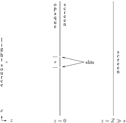
Figure \( 13.1\): The double slit experiment.

Now an interesting thing happens at the second screen, at \(z = Z\). This “screen” could be a photographic plate, a translucent screen, or even your retina. What appears on this screen is a series of parallel lines of brightness in the \(y\) direction (parallel to the slits). If one of the slits is covered up, the lines disappear.

What is going on is interference between the two possible straight-line paths by which the light can reach the screen. We will give a heuristic, physical discussion of the interference in this section. Then in the next section, we will derive the same result using the kind of forced oscillation and boundary condition arguments that you know from our study of one-dimensional waves.

The physical picture is this. The electric field at \(z = Z\) is a sum of the fields that come from the two slits. At \(x = 0\), in the symmetrical arrangement shown in Figure \( 13.1\), the two possible paths for the light have the same length. Therefore, the two components of the field have the same phase. Therefore they interfere “constructively” and there is a bright line at \(x = 0\). As x changes, at \(z = Z\), the relative length of the two paths changes. We will then get alternating positions of constructive and destructive interference. This gives rise to the bright lines.

We can understand the effect quantitatively by computing the path length explicitly. Consider a point on the screen at \(x = X\). This is shown in Figure \( 13.2\).

The length of the dotted line in Figure \( 13.2\) is \[\sqrt{X^{2}+Z^{2}}.\]

For the upper and lower slits, the path lengths are slightly shorter and longer respectively. The total difference in path length is \[\Delta \ell=\sqrt{(X+s / 2)^{2}+Z^{2}}-\sqrt{(X-s / 2)^{2}+Z^{2}}.\]

For \(Z \gg s\), we can expand \(\Delta \ell\) in (13.2) in a Taylor series, \[\Delta \ell \approx \frac{s X}{\sqrt{X^{2}+Z^{2}}}.\)

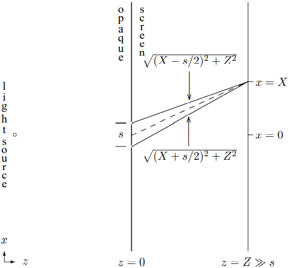
Figure \( 13.2\): Path lengths.

Therefore if the angular wave number of the light is \(k\), the phase difference between the two paths is \[\frac{k s X}{\sqrt{X^{2}+Z^{2}}}.\]

We get an intensity maximum every time the phase is a multiple of \(2 \pi\), when \[\frac{k s X}{\sqrt{X^{2}+Z^{2}}}=2 n \pi\]

In terms of the wavelength, \(\lambda=2 \pi / k\), this is \[\frac{X}{\sqrt{X^{2}+Z^{2}}}=n \frac{\lambda}{s}.\]

Fourier Optics

Suppose that instead of a simple pattern of two slits, there is some more complicated pattern on the opaque screen. In general, we can describe the wave disturbance in the \(z = 0\) plane by some function of \(x\) and \(y,^{1}\) \[f(x, y).\]

Our strategy will be to think of the wave produced for \(z > 0\) by this general function as a sum of the effects of tiny holes at all the values of \(x\) and \(y\) for which \(f(x, y)\) is nonzero. For each little piece of the function, we can compute the path length to some point on the screen at \(z = Z\). Then we can add up all the pieces.

Suppose, for simplicity, that \(f(x, y)\) is only nonzero in some small region around the origin, so that \(x\) and \(y\) will be small \[x, y \ll Z\]

for all relevant values of \(x\) and \(y\). Now the path length from the point \((x, y, 0)\) on the screen at \(z = 0\) to the point \((X, Y,Z)\) on the screen at \(z = Z\) is \[\sqrt{(X-x)^{2}+(Y-y)^{2}+Z^{2}}.\]

Using (13.8), we can expand this as follows: \[R+\Delta \ell(x, y)+\cdots ,\]

where \[R=\sqrt{X^{2}+Y^{2}+Z^{2}}\]

and \[\Delta \ell(x, y)=-\frac{x X+y Y}{R}\]

Thus the wave on the path from \((x, y, 0)\) to \((X, Y,Z)\) gets a phase of approximately \[e^{i k(R+\Delta \ell)}.\]

Now we can put the pieces of the wave back together to see how the interference works at the point \((X, Y,Z)\). We just sum over all values of \(x\) and \(y\), with a factor of the phase and the function, \(f(x, y)\). Because \(x\) and \(y\) are continuous variables, the sum is actually an integral, \[\int d x \int d y f(x, y) e^{i k(R+\Delta \ell)}=e^{i k R} \int d x \int d y f(x, y) e^{-i(x X+y Y) k / R}.\]

As we will see in more detail below, this is a two-dimensional Fourier transform of the function, \(f(x, y)\).

The equation, (13.14), is the fundamental result of Fourier optics. It contains much of the physics of diffraction. We have made a number of assumptions in deriving it that need further discussion. In the next section, we will derive it in a different way, treating the wave for \(z > 0\) as the result of a forced oscillation, produced by the wave in the \(z = 0\) plane. This will give us an alternative physical description of diffraction. But it will be useful to keep the simple picture of adding up all the possible paths in mind as we get deeper into the phenomena of interference and diffraction.

_________________________________

¹We are ignoring polarization.