3.10: Coaxial Line

Coaxial transmission lines consists of metallic inner and outer conductors separated by a spacer material as shown in Figure $\PageIndex{1}$. The spacer material is typically a low-loss dielectric material having permeability approximately equal to that of free space ($\mu\approx\mu_0$) and permittivity $\epsilon_s$ that may range from very near $\epsilon_0$ (e.g., air-filled line) to 2–3 times $\epsilon_0$. The outer conductor is alternatively referred to as the “shield,” since it typically provides a high degree of isolation from nearby objects and electromagnetic fields. Coaxial line is single-ended¹ in the sense that the conductor geometry is asymmetric and the shield is normally attached to ground at both ends. These characteristics make coaxial line attractive for connecting single-ended circuits in widely-separated locations and for connecting antennas to receivers and transmitters.

Figure $\PageIndex{1}$: Cross-section of a coaxial transmission line, indicating design parameters.

Coaxial lines exhibit TEM field structure as shown in Figure $\PageIndex{2}$.

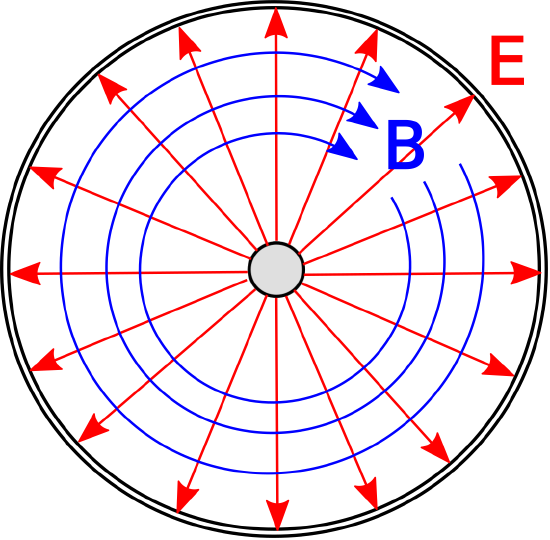Figure $\PageIndex{2}$: Structure of the electric and magnetic fields within coaxial line. In this case, the wave is propagating away from the viewer.

Expressions for the equivalent circuit parameters $C'$ and $L'$ for coaxial lines can be obtained from basic electromagnetic theory. It is shown in Section 5.24 that the capacitance per unit length is $$C' = \frac{2\pi\epsilon_s}{\ln\left(b/a\right)} \label{m0143_eCp}$$ where $a$ and $b$ are the radii of the inner and outer conductors, respectively. Using analysis shown in Section 7.14, the inductance per unit length is

$$L' = \frac{\mu_0}{2\pi}\ln\left(\frac{b}{a}\right) \label{m0143_eLp}$$

The loss conductance $G'$ depends on the conductance $\sigma_s$ of the spacer material, and is given by $$G' = \frac{2\pi\sigma_s}{\ln\left(b/a\right)} \nonumber$$ This expression is derived in Section 6.5.

The resistance per unit length, $R'$, is relatively difficult to quantify. One obstacle is that the inner and outer conductors typically consist of different materials or compositions of materials. The inner conductor is not necessarily a single homogeneous material; instead, the inner conductor may consist of a variety of materials selected by trading-off between conductivity, strength, weight, and cost. Similarly, the outer conductor is not necessarily homogeneous; for a variety of reasons, the outer conductor may instead be a metal mesh, a braid, or a composite of materials. Another complicating factor is that the resistance of the conductor varies significantly with frequency, whereas $C'$, $L'$, and $G'$ exhibit relatively little variation from their electro- and magnetostatic values. These factors make it difficult to devise a single expression for $R'$ that is both as simple as those shown above for the other parameters and generally applicable. Fortunately, it turns out that the low-loss conditions $R'\ll\omega L'$ and $G'\ll\omega C'$ are often applicable,² so that $R'$ and $G'$ are important only if it is necessary to compute loss.

Since the low-loss conditions are often met, a convenient expression for the characteristic impedance is obtained from Equations $\ref{m0143_eCp}$ and $\ref{m0143_eLp}$ for $L'$ and $C'$ respectively:

$$\begin{aligned} Z_{0} & \approx \sqrt{\frac{L^{\prime}}{C^{\prime}}}(\text { low-loss }) \\ &=\frac{1}{2 \pi} \sqrt{\frac{\mu_{0}}{\epsilon_{s}}} \ln \frac{b}{a} \end{aligned}$$

The spacer permittivity can be expressed as $\epsilon_s=\epsilon_r\epsilon_0$ where $\epsilon_r$ is the relative permittivity of the spacer material. Since $\sqrt{\mu_0/\epsilon_0}$ is a constant, the above expression is commonly written $$Z_0 \approx \frac{60~\Omega}{\sqrt{\epsilon_r}} \ln{\frac{b}{a}} ~~~\mbox{(low-loss)} \nonumber$$ Thus, it is possible to express $Z_0$ directly in terms of parameters describing the geometry ($a$ and $b$) and material ($\epsilon_r$) used in the line, without the need to first compute the values of components in the lumped-element equivalent circuit model.

Similarly, the low-loss approximation makes it possible to express the phase velocity $\nu_p$ directly in terms the spacer permittivity:

$$\begin{aligned} \nu_{p} & \approx \frac{1}{\sqrt{L^{\prime} C^{\prime}}} \text { (low-loss) } \\ &=\frac{c}{\sqrt{\epsilon_{r}}} \end{aligned}$$

since $c\triangleq 1/\sqrt{\mu_0\epsilon_0}$. In other words, the phase velocity in a low-loss coaxial line is approximately equal to the speed of electromagnetic propagation in free space, divided by the square root of the relative permittivity of the spacer material. Therefore, the phase velocity in an air-filled coaxial line is approximately equal to speed of propagation in free space, but is reduced in a coaxial line using a dielectric spacer.

Example $\PageIndex{1}$: RG-59 Coaxial Cable

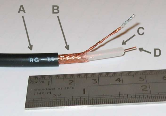Figure $\PageIndex{3}$: RG-59 coaxial line. A: Insulating jacket. B: Braided outer conductor. C: Dielectric spacer. D: Inner conductor (© CC BY SA 3.0; Arj)

RG-59 is a very common type of coaxial line. Figure $\PageIndex{3}$ shows a section of RG-59 cut away so as to reveal its structure. The radii are $a\cong 0.292$ mm and $b\approx 1.855$ mm (mean), yielding $L'\approx 370$ nH/m. The spacer material is polyethylene having $\epsilon_r\cong 2.25$, yielding $C'\approx 67.7$ pF/m. The conductivity of polyethylene is $\sigma_s\cong 5.9 \times 10^{-5}$ S/m, yielding $G'\approx 200~\mu$S/m. Typical resistance per unit length $R'$ is on the order of $0.1~\Omega$/m near DC, increasing approximately in proportion to the square root of frequency.

From the above values, we find that RG-59 satisfies the low-loss criteria $R'\ll\omega L'$ for $f\gg 43$ kHz and $G'\ll\omega C'$ for $f\gg 470$ kHz. Under these conditions, we find $Z_0 \approx \sqrt{L'/C'} \cong 74~\Omega$. Thus, the ratio of the potential to the current in a wave traveling in a single direction on RG-59 is about $74~\Omega$.

The phase velocity of RG-59 is found to be $v_p \approx 1/\sqrt{L'C'} \cong 2 \times 10^8$ m/s, which is about 67% of $c$. In other words, a signal that takes 1 ns to traverse a distance $l$ in free space requires about 1.5 ns to traverse a length-$l$ section of RG-59. Since $v_p = \lambda f$, a wavelength in RG-59 is 67% of a wavelength in free space.

Using the expression $$\gamma = \sqrt{\left(R'+j\omega L'\right)\left(G'+j\omega C'\right)} \nonumber$$ with $R'=0.1~\Omega$/m, and then taking the real part to obtain $\alpha$, we find $\alpha\sim 0.01$ m$^{-1}$. So, for example, the magnitude of the potential or current is decreased by about 50% by traveling a distance of about 70 m. In other words, $e^{-\alpha l} = 0.5$ for $l \sim 70$ m at relatively low frequencies, and increases with increasing frequency.

Additional Reading:

• “Coaxial cable” on Wikipedia. Includes descriptions and design parameters for a variety of commonly-encountered coaxial cables.
• “Single-ended signaling” on Wikipedia.
• Sec. 8.7 (“Differential Circuits”) in S.W. Ellingson, Radio Systems Engineering, Cambridge Univ. Press, 2016.

---

1. The references in “Additional Reading” at the end of this section may be helpful if you are not familiar with this concept.↩
2. See Section 3.9 for a reminder about this concept.↩