7.4: Calculating Work Numerically

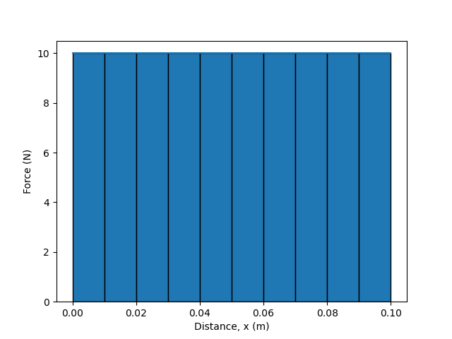
It's possible, many students in Physics 1 have not had Calculus 2, and integrals are not familiar. Let's take a graphical look at the work. In Figure \(\PageIndex{1}\), a constant \(10~ \text{N}\) net force is moving an object at constant velocity over a distance of \(0.1~ \text{m}\). The action is split into ten segments. Considering the relationship

$$W = \vec{F}\cdot\vec{d}$$

we can see that when the force and displacement are aligned, the work is \(W=\left|\vec{F}\right|\left|\vec{d}\right| = Fd\). This is the height times width, or area, of the graph. We could break the graph into segments and add the segments. As described in the previous section, the area of the segments can be written \(\vec F_i \cdot \Delta \vec x\) and summed to obtain the full area of the graph of \(F\) vs. \(x\).

\begin{align*} W^{tot} = \sum_{i=0}^N\vec F_i \cdot \Delta \vec x_i \end{align*}

Figure \(\PageIndex{1}\): A constant net force of 10 Newtons applied to an object moving a of 0.1 meter.

 

Example \(\PageIndex{2}\)

A block is pushed with \(10\) Newtons of net force to move the block with constant velocity \(0.1\) meters. Split the work into intervals of \(\Delta x = 0.01\) meters and calculate the total work done as the sum of the work over all of the intervals.

Solution

Let's make a table of all of the intervals.

\(F_i\) (N)	\(\Delta~x\) (m)	\(W_i\) (J)
\(10\)	\(0.01 - 0.00 = 0.01\)	\(10 \times 0.01 = 0.1\)
\(10\)	\(0.02 - 0.01 = 0.01\)	\(10 \times 0.01 = 0.1\)
\(10\)	\(0.03 - 0.02 = 0.01\)	\(10 \times 0.01 = 0.1\)
\(10\)	\(0.04 - 0.03 = 0.01\)	\(10 \times 0.01 = 0.1\)
\(10\)	\(0.05 - 0.04 = 0.01\)	\(10 \times 0.01 = 0.1\)
\(10\)	\(0.06 - 0.05 = 0.01\)	\(10 \times 0.01 = 0.1\)
\(10\)	\(0.07 - 0.06 = 0.01\)	\(10 \times 0.01 = 0.1\)
\(10\)	\(0.08 - 0.07 = 0.01\)	\(10 \times 0.01 = 0.1\)
\(10\)	\(0.09 - 0.08 = 0.01\)	\(10 \times 0.01 = 0.1\)
\(10\)	\(0.1 - 0.09 = 0.01\)	\(10 \times 0.01 = 0.1\)

Now, we can simply add the last column on the right.

\begin{align*}
W^{tot} &= \sum_{i=0}^N\vec F_i \cdot \Delta \vec x_i \\
&= 0.1 + 0.1 + 0.1 + 0.1 + 0.1 + 0.1 + 0.1 + 0.1 + 0.1 + 0.1\\
&= 1~\text{J}
\end{align*}

Notice that this is the same as
$$W^{tot} = Fd = 10\cdot 0.1 = 1~\text{J}$$

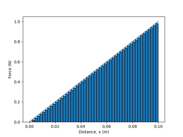
Next, let's look at the spring example from the previous section. Instead of compressing the spring we will consider stretching the spring in the \(+\hat{x}\)-direction. The force applied to stretching the spring is \(\vec{F}=kx \hat{x}\). If we plot \(F\) vs. \(x\) for stretching a spring with spring constant \(k=10~\text{N/m}\) from \(x=0\) to \(x=0.1\) meters, we get the graph shown in Figure  \(\PageIndex{3}\). We can see that the force increases linearly with displacement. When we divide the displacement into intervals, we no longer can fit rectangular areas to fully describe the area of the force vs. displacement. That is okay, we can approximate the area with these rectangular areas.

Figure \(\PageIndex{3}\): Force vs. displacement for stretching a spring with k=10 N/m a distance of 0.1 meter. The graph is split into 10 segments.

Example \(\PageIndex{4}\)

A spring with spring constant \(k=10~\text{N/m}\) is stretched from its equilibrium length \(x=0~\text{m}\) by an amount \(x=0.1~\text{m}\). Use the numerical summation described above to find the work done stretching the spring. Use the value of the force at the left edge of the rectangular segments as shown in Figure \(PageIndex{3}\).

Solution

Let's make a table of all of the intervals.

\(F_i = kx_i\) (N)	\(\Delta~x\) (m)	\(W_i\) (J)
\(10\times 0.00 = 0.00\)	\(0.01 - 0.00 = 0.01\)	\(0.00 \times 0.01 = 0.000\)
\(10\times 0.01 = 0.10\)	\(0.02 - 0.01 = 0.01\)	\(0.10 \times 0.01 = 0.001\)
\(10\times 0.02 = 0.20\)	\(0.03 - 0.02 = 0.01\)	\(0.20 \times 0.01 = 0.002\)
\(10\times 0.03 = 0.30\)	\(0.04 - 0.03 = 0.01\)	\(0.30 \times 0.01 = 0.003\)
\(10\times 0.04 = 0.40\)	\(0.05 - 0.04 = 0.01\)	\(0.40 \times 0.01 = 0.004\)
\(10\times 0.05 = 0.50\)	\(0.06 - 0.05 = 0.01\)	\(0.50 \times 0.01 = 0.005\)
\(10\times 0.06 = 0.60\)	\(0.07 - 0.06 = 0.01\)	\(0.60 \times 0.01 = 0.006\)
\(10\times 0.07 = 0.70\)	\(0.08 - 0.07 = 0.01\)	\(0.70 \times 0.01 = 0.007\)
\(10\times 0.08 = 0.80\)	\(0.09 - 0.08 = 0.01\)	\(0.80 \times 0.01 = 0.008\)
\(10\times 0.09 = 0.90\)	\(0.1 - 0.09 = 0.01\)	\(0.90 \times 0.01 = 0.009\)

Now, we can simply add the last column on the right.

\begin{align*}
W^{tot} &= \sum_{i=0}^N\vec F_i \cdot \Delta \vec x_i \\
&= 0.000 + 0.001 + 0.002 + 0.003 + 0.004 + 0.005 + 0.006 + 0.007 + 0.008 + 0.009\\
&= 0.045~\text{J}
\end{align*}

Let's compare to the work computed from integration in the previous section.

$$W^{tot} = \frac{1}{2}kx^2 = \frac{1}{2}10\cdot\left(0.1\right)^2 = 0.05~\text{J}$$

So, our approximation is close. You might notice that the area of this graph is a triangle, and we could calculate

\begin{align*}
W &= A_{triangle}\\
&= \frac{1}{2}\text{base} \cdot~\text{height} \\
&= \frac{1}{2}Fx \\
&= \frac{1}{2}kx \cdot x \\
&= \frac{1}{2}kx^2
\end{align*}

We could improve our approximation by dividing the \(F\) vs. \(x\) graph into smaller intervals as shown in Figure \(\PageIndex{5}\). The calculation using a table would be tedious. Let's see how a computer can help us solve this problem.

Figure \(\PageIndex{5}\): Force vs. displacement for stretching a spring with k=10 N/m a distance of 0.1 meter. The graph is split into 50 segments.

 

In the trinket below we will compute the spring force as a function of stretch distance. First, we should define some variables such as the spring constant \(k\), the total stretch distance \(x\), the intervals of stretch \(\Delta x\), and the work \(W\). The total distance and the work are going to be summed in a loop. So, we initialize them to zero. We'll begin by repeating the calculation above to make sure we get the expected results.

k = 10 #spring constant in N/m
x = 0 #total stretch distance
dx = 0.01 #stretch interval
W = 0

 

Next, we will create a loop that continues while the stretch is less than \(0.1\) meters. This should make the last left edge be \(x=0.09\) and the last \(\Delta x = 0.1-0.09\). Inside that loop we want to calculate the force at the left side of the rectangle (this is \(x\). Then, add the work this force does over the increment of displacement \(F\Delta x\) to the work that has been done in previous increments of displacement. We'll print the results that are in the table above, and we can't forget to increment \(x\) for the next loop.

while x < 0.1:
    rate(2)
    F = k*x #force at left side of interval
    W = W + F*dx
    print(x, F, W)
    x = x + dx

Run this code to see that it works to produce the values in the table above. If you want to create more intervals, you only need to decrease the value of \(\Delta x\) or dx in your code. Try changing this value to dx=0.005 (20 intervals). Then, try dx = 0.001. Does this make the summation closer to the exact value of \(W=\frac{1}{2}kx^2=0.05~\text{J}\)? How small does dx need to be to be within 1% of the exact value?

For fun, we can graph and simulate the scenario of stretching a spring. To create a graph add the following two lines after the Web VPython 3.2 line. This will create a graph and f1 is the data that is displayed on the graph.

spring_graph = graph(xtitle='x (m)', ytitle='W (J)')
f1 = gdots(color=color.red) 

On the line after the calculation of work in the loop, add the following line to put position on the x-axis and work on the y-axis. This will add a single point to the graph each time the loop iterates.

f1.plot(x, W) #add this data point to a graph 

Check that this works properly in your trinket. Once that works, you can add an object simulation. After the line with f1, create a spring with the following code.

spring = helix(pos=vec(-0.125, 0, 0), axis=vec(0.25, 0, 0), radius=0.1, coils = 3)

After the line where the work is calculated, add the following line to extend the spring from its equilibrium length to the equilibrium length plus \(x\).

spring.axis=vec(0.25+x, 0, 0)