16.3: The Electric Field

We define the electric field vector, $\vec E$, in an analogous way as we defined the gravitational field vector, $\vec g$. By defining the gravitational field vector, say, at the surface of the Earth, we can easily calculate the gravitational force exerted by the Earth on any mass, $m$, without having to use Newton’s Universal Theory of Gravity. As you recall, we can define the gravitational field, $\vec g(\vec r)$, at some position, $\vec r$, from a point mass, $M$, as the gravitational force per unit mass:

$$\begin{aligned} \vec g(\vec r) = -G \frac{M}{r^2}\hat r\end{aligned}$$

where $\vec r$ is a vector from the position of $M$ to where we want to know the gravitational field. As a result, the force exerted on a “test mass”, $m$, located at position $\vec r$ relative to mass $M$ is given by:

$$\begin{aligned} \vec F^g=m\vec g= -G\frac{Mm}{r^2}\hat r\end{aligned}$$

which, of course, is the result from Newton’s Theory of Gravity. As you recall, we can define the gravitational field for any object that is not a point mass (e.g. the Earth), and use that field to find the force exerted by the Earth on any mass $m$, without having to re-calculate the gravitational field each time (which requires an integral or Gauss’ Law).

We proceed in an analogous was to define the “Electric field”, $\vec E(\vec r)$, as the electric force per unit charge. If we have a point charge, $Q$, located at the origin of a coordinate system, then the electric field from that point charge, $\vec E(\vec r)$, at some position, $\vec r$, relative to the origin is given by:

 

$$\vec E(\vec r)=k\frac{Q}{r^{2}}\hat r$$

If we place a “test charge”, $q$, at position $\vec r$ in space, it will experience a force given by:

$$\begin{aligned} \vec F^e=q\vec E=k\frac{Qq}{r^2}\hat r\end{aligned}$$

just as we find from Coulomb’s Law.

Exercise $\PageIndex{1}$

A negative charge is placed at the origin of a coordinate system. At some point in space, the electric field from that charge

1. points towards the origin.
2. points away from the origin.

Answer

A.

In Example 16.2.2, we determined the electric force on charge $q$, exerted by two other charges $Q_1$ and $Q_2$. If we now changed the value of $q$ and wanted to determine the force, we can use the electric field to simplify the process considerably. That is, we can determine the value of the electric field, $\vec E$, from $Q_1$ and $Q_2$ at the position of $q$, and then simply multiply that field vector by a charge $q$ to obtain the force on that charge, without having to add force vectors.

Example $\PageIndex{1}$

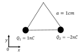
Two charges, \(Q_1=1\text{nC}\), and $Q_2=-2\text{nC}$ are held fixed at two corners of an equilateral triangle with sides of length $a=1\text{cm}$, with a coordinate system as shown in Figure $\PageIndex{2}$. What is the electric field vector at the third corner of the triangle?

Figure $\PageIndex{1}$: Two charges at the corners of an equilateral triangle of side $a$.

Solution

The net electric field at the third corner of the triangle will be the vector sum of the electric fields from charges $Q_1$ and $Q_2$. We thus need to determine the electric field vectors from each charge, and then add those two vectors to obtain the net electric field. The vectors are illustrated in Figure $\PageIndex{2}$.

Figure $\PageIndex{2}$: Electric field vectors from two charges at the corners of an equilateral triangle of side $a$.

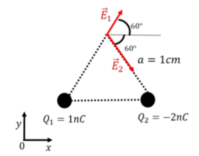
The electric field from charge $Q_1$ has magnitude:

$$\begin{aligned} E_1=\left |k\frac{Q_1}{a^2}\right |=(9\times 10^{9}\text{N}\cdot \text{m}^2\text{/C}^{2})\frac{(1\times 10^{-9}\text{C})}{(0.01\text{m})^2}=9\times 10^{4}\text{N/C}\end{aligned}$$

and components:

$$\begin{aligned} \vec E_1&=E_1\cos(60^{\circ})\hat x+E_1\sin(60^{\circ})\hat y\\[4pt] &=(4.5\times 10^{4}\text{N/C})\hat x+(7.8\times 10^{4}\text{N/C})\hat y\end{aligned}$$

Similarly, the electric field from $Q_2$ has magnitude:

$$\begin{aligned} E_2=\left |k\frac{Q_2}{a^2}\right |=(9\times 10^{9}\text{N}\cdot \text{m}^2\text{/C}^{2})\frac{(2\times 10^{-9}\text{C})}{(0.01\text{m})^2}=1.8\times 10^{5}\text{N/C}\end{aligned}$$

and components:

$$\begin{aligned} \vec E_2&=E_2\cos(60^{\circ})\hat x-E_2\sin(60^{\circ})\hat y\\[4pt] &=(9.0\times 10^{4}\text{N/C})\hat x-(1.6\times 10^{5}\text{N/C})\hat y\end{aligned}$$

Finally, we can add the two force vectors together to obtain the net force on $q$:

$$\begin{aligned} \vec E^{net}&=\vec E_1+\vec E_2\\[4pt] &=(4.5\times 10^{4}\text{N/C})\hat x+(7.8\times 10^{4}\text{N/C})\hat y+(9.0\times 10^{4}\text{N/C})\hat x-(1.6\times 10^{5}\text{N/C})\hat y\\[4pt] &=(13.5\times 10^{4}\text{N/C})\hat x-(8.2\times 10^{4}\text{N/C})\hat y\end{aligned}$$

which has a magnitude of $15.8\times 10^{4}\text{N/C}$. By knowing the electric field at the empty corner of the triangle, we can now calculate the net electric force that would act on any charge placed in that location. For example, if we place a charge $q=-1\text{nC}$ (as in Example 16.2.2), we can easily find the corresponding electric force:

$$\begin{aligned} \vec F_q &= q\vec E=(-1\text{nC})\left[ (13.5\times 10^{4}\text{N/C})\hat x-(8.2\times 10^{4}\text{N/C})\hat y \right]\\[4pt] &=-(13.5\times 10^{-5}\text{N})\hat x+(8.2\times 10^{-5}\text{N})\hat y\end{aligned}$$

as we found previously. Note that the force on $q$ is in the opposite direction of the electric field vector. This is because $q$ is negative. The electric field at some point in space thus points in the same direction as the force that a positive test charge would experience.

Discussion

In this example, we determined the net electric field by making use of the superposition principle; namely, that we can treat the electric fields from $Q_1$ and $Q_2$ independently, without needing to consider the fact that $Q_1$ and $Q_2$ exert forces on each other. By knowing the electric field at some position in space, we can easily calculate the force vector on any test charge, $q$, placed at that position. Furthermore, the sign of the charge $q$ will determine in which direction the force will point (parallel to $\vec E$ for a positive charge and anti-parallel to $\vec E$ for a negative charge).

Exercise $\PageIndex{2}$

The electric field inside of a conductor must be zero because...

1. If there is an electric field, electrons will move (since it is a conductor) and arrange themselves so as to create an additional field that cancels the original field
2. If there is an electric field, protons will move (since it is a conductor) and arrange themselves so as to create an additional field that cancels the original field
3. Since electrons can move freely, they move so fast that the electric field is negligible.
4. Electric fields cannot penetrate conducting materials.

Answer

A.

Visualizing the electric field

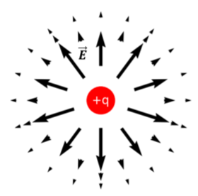
Generally, a “field” is something that has a different value at different positions in space. The pressure in a fluid under the presence of gravity is a field: the pressure is different at different heights in the fluid. Since pressure is a scalar quantity (a number), we call it a “scalar field”. The electric field is called a “vector field”, because it is a vector that is different at each position in space. One way to visualize the electric field is to draw arrows at different positions in space; the length of the arrow is then proportional to the strength of the electric field at that position, and the direction of the arrow then represents the direction of the electric field. The electric field for a point charge is shown using this method in Figure $\PageIndex{3}$.

Figure $\PageIndex{3}$: Electric field vectors near a point charge.

One disadvantage of visualizing a vector field with arrows is that the arrows take up space, and it can be challenging to visualize how the field changes magnitude and direction continuously through space. For this reason, one usually uses “field lines” to visualize a vector field. Field lines are continuous lines with the following properties:

• The direction of the vector field at some point in space is tangent to the field line at that point.
• Field lines have a direction to indicate the direction of the field vector along the tangent (as there are two possibilities, parallel and anti-parallel).
• The magnitude of the field is proportional to the density of field lines at that point. The more field lines near a location in space, the larger the magnitude of the field vector at that point.

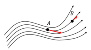
An example of using field lines to represent a vector field in space is shown in Figure $\PageIndex{4}$. The corresponding field vector is shown at two different positions in space ($A$ and $B$). At both positions, the vector is tangent to the field line at that position in space and points in the direction of the little arrow drawn at the end of the field lines. The field vector at point $A$ has a larger magnitude than the one at point $B$, since the field lines are more concentrated at point $A$ than at point $B$ (there are more field lines per unit area at that position in space, the field lines are closer together).

Figure $\PageIndex{4}$: An example of determining a field vector from the continuous field lines.

Exercise $\PageIndex{3}$

It is possible for field lines to cross?

1. Yes.
2. No.

Answer

B.

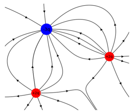
Because the electric field vector always points in the direction of the force that would be exerted on a positive charge, electric field lines will point out from a positive charge and into a negative charge. The electric field lines for a combination of positive and negative charges is illustrated in Figure $\PageIndex{5}$.

Figure $\PageIndex{5}$: Field lines of two $+2q$ charges and one $-3q$ charge.

Electric field from a charge distribution

So far, we have only considered Coulomb’s Law for point charges (charges that are infinitely small and can be considered to exist at a single point in space). We can use the principle of superposition to determine the electric field from a charged extended/continuous object by modeling that object as being made of many point charges. The electric field from that object is then the sum of the electric field from the point charges that make up that object.

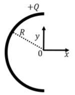
Consider a charged wire that is bent into a semi-circle of radius $R$, as in Figure $\PageIndex{6}$. The wire carries a net positive electric charge, $+Q$, that is uniformly distributed along the length of the wire. We wish to determine the electric field vector at the center of the circle.

Figure $\PageIndex{6}$: A charged wire bent into a semi-circle of radius $R$.

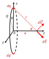
We start by choosing a very small section of wire and model that section of wire as a point charge with infinitesimal charge $dq$ (as in Figure $\PageIndex{7}$). A distance $R$ from that point charge, the electric field from that point charge will have magnitude, $dE$, given by:

$$\begin{aligned} dE=k\frac{dq}{R^2}\end{aligned}$$

The electric field vector, $d\vec E$, from the point charge $dq$ is illustrated in Figure $\PageIndex{7}$.

Figure $\PageIndex{7}$: Infinitesimal electric fields from point charges along the bent wire.

Using the coordinate system that is shown, we define $\theta$ as the angle made by the vector from the origin to the point charge $dq$ and the $x$-axis. The electric field vector from $dq$ is then given by:

$$\begin{aligned} d\vec E = dE\cos\theta \hat x - dE\sin\theta \hat y\end{aligned}$$

The total electric field at the origin will be obtained by summing the electric fields from the different $dq$ over the entire semi-circle:

$$\begin{aligned} \vec E &= \int d\vec E = \int \left(dE\cos\theta \hat x - dE\sin\theta \hat y\right)\\[4pt] &=\left( \int dE\cos\theta \right)\hat x -\left( \int dE\sin\theta \right)\hat y\\[4pt] \therefore E_x &= \int dE\cos\theta\\[4pt] \therefore E_y &= -\int dE\sin\theta\\[4pt]\end{aligned}$$

We are thus left with two integrals to solve for the $x$ and $y$ components of the electric field, respectively. Before jumping into solving the integrals, it is useful to think about the symmetry of the problem. Specifically, consider a second point charge, $dq'$, located symmetrically about the $x$-axis from charge $dq$, as illustrated in Figure $\PageIndex{7}$. The charge $dq'$ will create a small electric field $d\vec E'$ as illustrated. When we add together $d\vec E$ and $d\vec E'$, the two $y$ components will cancel, and only the $x$ components will sum together. Similarly, for any $dq$ that we choose, there will always be another $dq'$ such that when we sum together their respective electric fields, the $y$ components will cancel. Thus, by symmetry, we can argue that the net $y$ component of the electric field, $E_y$, must be identically zero. We thus only need to evaluate the $x$ component of $\vec E$:

$$\begin{aligned} E_x = \int dE\cos\theta = \int k\frac{dq}{R^2} \cos\theta\end{aligned}$$

In order to solve this integral, we need to consider which variables change for different choices of the point charge $dq$. In this case, the distance $R$ is the same anywhere along the semi-circle, so only $\theta$ changes with different choices of $dq$, as $k$ is a constant. We can express $dq$ in terms of $d\theta$ and then use $\theta$ as the variable of integration (the variable that labels the different $dq$). $d\theta$ corresponds to a small change in the angle $\theta$, and is the angle that is subtended by the charge $dq$. That is, the charge $dq$ covers a small arc length, $ds$, of the semi-circle, which is related to $d\theta$ by:

$$\begin{aligned} ds = Rd\theta\end{aligned}$$

The total charge on the wire is given by $Q$, and the wire has a length $\pi R$ (half the circumference of a circle). Since the charge is distributed uniformly on the wire, the charge per unit length of any piece of wire must be constant. In particular, $dq$ divided by $ds$ must be equal to $Q$ divided by $\pi R$:

$$\begin{aligned} \frac{dq}{ds}&=\frac{Q}{\pi R}\\[4pt] \therefore dq &=\frac{Q}{\pi R}ds=\frac{Q}{\pi}d\theta\end{aligned}$$

where in the last equality we used the relation $ds=Rd\theta$. We now have all of the ingredients to solve the integral:

$$\begin{aligned} E_x &= \int k\frac{dq}{R^2} \cos\theta = \int_{-\pi/2}^{+\pi/2} k\frac{Q}{\pi R^2}\cos\theta d\theta\\[4pt] &= k\frac{Q}{\pi R^2}\int_{-\pi/2}^{+\pi/2}\cos\theta d\theta=k\frac{Q}{\pi R^2}\left[ \sin\theta \right]_{-\pi/2}^{+\pi/2}\\[4pt] &= k\frac{2Q}{\pi R^2}\end{aligned}$$

The total electric field vector at the center of the circle is thus given by:

$$\begin{aligned} \vec E = k\frac{2Q}{\pi R^2} \hat x\end{aligned}$$

Note that if we had not realized that we did not need to solve the integral for the $y$ component, we would still find that it is zero:

$$\begin{aligned} E_y= -k\frac{Q}{\pi R^2}\int_{-\pi/2}^{+\pi/2}\cos\theta d\theta=-k\frac{Q}{\pi R^2}\left[ -\cos\theta \right]_{-\pi/2}^{+\pi/2}=0\end{aligned}$$

In order to determine the electric field at some point from any continuous charge distribution, the procedure is generally the same:

1. Make a good diagram.
2. Choose a charge element $dq$.
3. Draw the electric field element, $d\vec E$, at the point of interest.
4. Write out the electric field element vector, $d\vec E$, in terms of $dq$ and any other relevant variables.
5. Think of symmetry: will any of the component of $d\vec E$ sum to zero over all of the $dq$?
6. Write the total electric field as the sum (integral) of the electric field elements.
7. Identify which variables change as one varies the $dq$ and choose an integration variable to express $dq$ and everything else in terms of that variable and other constants.
8. Do the sum (integral).

Example $\PageIndex{2}$

A ring of radius $R$ carries a total charge $+Q$. Determine the electric field a distance $a$ from the center of the ring, along the axis of symmetry of the ring.

Solution

In order to determine the electric field, we carry out the procedure outlined above, and start by drawing a good diagram, as in Figure $\PageIndex{8}$, showing: our coordinate system, our choice of $dq$, the electric field element vector $d\vec E$ that corresponds to $dq$, and variables ($r$, $\theta$) to specify the position of $dq$.

Figure $\PageIndex{8}$: Determining the electric field on the axis of a ring of radius $R$ carrying charge $Q$.

In this case, the figure is challenging to draw and visualize because of the three-dimensional nature of the problem. With the specific $dq$ that we chose, the electric field element vector is given by:

$$\begin{aligned} d\vec E = -dE\sin\theta \hat x + 0\hat y + dE\cos\theta \hat z \end{aligned}$$

where $d\vec E$ has magnitude:

$$\begin{aligned} dE = k\frac{dq}{r^2}\end{aligned}$$

The $x$ and $z$ components of the total electric field will then be given by:

$$\begin{aligned} E_x &= -\int dE\sin\theta=-\int k\frac{dq}{r^2}\sin\theta\\[4pt] E_z &= \int dE\cos\theta=\int k\frac{dq}{r^2}\cos\theta \\[4pt]\end{aligned}$$

In general, if we had chosen a $dq$ that is not along one of the axes of the coordinate system, the electric field element vector would have components in all three directions. However, if we consider the symmetry of the ring, we can note that once we sum together all of the electric field elements, only the $z$ components will survive. Indeed, we have shown in Figure $\PageIndex{8}$ that for each $dq$, there will be a $dq'$ located on the opposite side of the ring that will create an electric field element that will cancel all but the $z$ component of the field element from $dq$. We thus only need to consider the $z$ components of the electric field elements when determining the total electric field:

$$\begin{aligned} \vec E = E_z\hat z\end{aligned}$$

We now have to evaluate the integral for the $z$ component of the electric field:

$$\begin{aligned} E_z &= \int k\frac{dq}{r^2}\cos\theta \\[4pt]\end{aligned}$$

and determine which quantities change as we move $dq$ around the ring. In this case, both $r^2$ and $\cos\theta$ are the same for all elements on the ring, and the integral is trivial:

$$\begin{aligned} E_z &= k\frac{1}{r^2}\cos\theta\int dq=k\frac{Q}{r^2}\cos\theta=kQ\frac{a}{(R^2+a^2)^\frac{3}{2}} \\[4pt]\end{aligned}$$

where the integral $\int dq$ simply means “sum all of the charges $dq$ together”, which is equal to $Q$, the total charge on the ring. In the last equality, we replaced $\cos\theta$ with the variables $a$ and $R$ that are provided in the question.

Example $\PageIndex{3}$

You have rubbed a glass rod with a silk cloth such that the glass rod has acquired a positive charge. The rod has a length, $L$, a negligible cross-section, and has acquired a total positive charge, $+Q$, that is uniformly distributed along the length of the rod. What is the electric field a distance $R$ from the center of the rod?

Solution

In order to determine the electric field, we carry out the procedure outlined above, and start by drawing a good diagram, as in Figure $\PageIndex{9}$, showing: our coordinate system, our choice of $dq$ at a distance $y$ above the center of the rod, the electric field element vector $d\vec E$ that corresponds to $dq$, and variables ($y$, $r$, $\theta$) to specify the position of $dq$.

Figure $\PageIndex{9}$: Determining the electric field a distance $R$ from the center of a rod of length $L$ carrying charge $Q$.

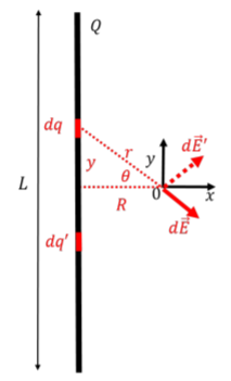
We define the origin to be located at the point where we want to determine the electric field, and the angle $\theta$ to be the angle between the horizontal and the position vector of $dq$. We can write the electric field element vector as:

$$\begin{aligned} d\vec E = dE\cos\theta \hat x - dE\sin\theta \hat y\end{aligned}$$

where $d\vec E$ has magnitude:

$$\begin{aligned} dE = k\frac{dq}{r^2}\end{aligned}$$

The $x$ and $y$ components of the total electric field will then be given by:

$$\begin{aligned} E_x &= \int dE\cos\theta=\int k\frac{dq}{r^2}\cos\theta \\[4pt] E_y &= -\int dE\sin\theta=-\int k\frac{dq}{r^2}\sin\theta\\[4pt]\end{aligned}$$

Again, before proceeding with the integrals, we consider symmetry. Specifically, if we consider a charge $dq'$ located symmetrically about the $x$ axis from $dq$ (as illustrated in Figure $\PageIndex{9}$), we see that the $y$ component of the electric field element $d\vec E'$ that it creates will cancel the $y$ component of $d\vec E$. For each choice of $dq$, there will exist a corresponding choice $dq'$ which will result in the $y$ component of the net electric field being zero. We thus only need to evaluate the $x$ component of the total electric field:

$$\begin{aligned} \vec E = E_x \hat x = \left(\int k\frac{dq}{r^2}\cos\theta\right) \hat x\end{aligned}$$

Within the integrand, both $r$ and $\theta$ will change as we sum over the different charges $dq$ along the rod. A straightforward option to write the integral is to use $y$ as the integration constant, and to write $dq$, $r$, and $\cos\theta$ in terms of $y$. The charge $dq$ covers an infinitesimal length of the rod, $dy$. Since the rod is uniformly charged, the charge per unit length must be the same over a small length $dy$ as it is over the whole length of the rod:

$$\begin{aligned} \frac{dq}{dy}&=\frac{Q}{L}\\[4pt] \therefore dq &= \frac{Q}{L} dy\end{aligned}$$

It is often useful to introduce a constant charge per unit length, $\lambda=\frac{Q}{L}$, so that we can write the charge $dq$ as:

$$\begin{aligned} dq = \lambda dy\end{aligned}$$

We can also express $r^2$ and $\cos\theta$ in terms of $y$ (and $R$, which is constant):

$$\begin{aligned} r^2 &= y^2+R^2\\[4pt] \cos\theta&=\frac{R}{r}=\frac{R}{\sqrt{y^2+R^2}}\end{aligned}$$

Finally, we can combine this all into an integral that we can evaluate:

$$\begin{aligned} E_x &=\int k\frac{dq}{r^2}\cos\theta\\[4pt] &=k\int_{-L/2}^{L/2} \lambda \frac{1}{y^2+R^2}\frac{R}{\sqrt{y^2+R^2}} dy\\[4pt] &=kR\lambda\int_{-L/2}^{L/2} \frac{1}{(y^2+R^2)^{\frac{3}{2}}} dy\\[4pt] &=kR\lambda \left[ \frac{y}{R^2\sqrt{y^2+R^2}}\right]_{-L/2}^{L/2}\\[4pt] \therefore E_x &= \frac{k\lambda}{R}\frac{L}{\sqrt{\left(\frac{L}{2}\right)^2+R^2}} \end{aligned}$$

If the rod were infinitely long (or very long compared to the distance $R$), the electric field becomes:

$$\begin{aligned} \lim_{L\to\infty}E_x=\frac{2k\lambda}{R}\end{aligned}$$

By using the charge per unit length, $\lambda$, we were able to easily generalize our result to that expected for an infinitely long rod with uniform charge density.

Solving the integral above in terms of the integration variable $y$ is difficult without some knowledge of integrals. For this specific integral, the easiest method to use from calculus is “trig substitution”. We show below how we can arrive at a much easier integral if we had instead chosen the angle $\theta$ as the integration variable instead of $y$, and we will see that this is a physical illustration of the “trig substitution method” from calculus!

We go back to step 7 in our procedure and choose $\theta$ (instead of $y$) as the integration variable for the integral:

$$\begin{aligned} E_x &=\int k\frac{dq}{r^2}\cos\theta\\[4pt]\end{aligned}$$

That is, we need to express $1/r^2$ and $dq$ in terms of $\theta$. Referring to Figure $\PageIndex{9}$, we have:

$$\begin{aligned} r &= \frac{R}{\cos\theta}\\[4pt] \therefore \frac{1}{r^2}&=\frac{\cos^2\theta}{R^2}\\[4pt] y &= R\tan\theta\\[4pt] \therefore dy &= \frac{dy}{d\theta}d\theta=\frac{R}{\cos^2\theta}d\theta\\[4pt] \therefore dq &= \lambda dy =\lambda\frac{R}{\cos^2\theta}d\theta\end{aligned}$$

The only difficulty is in determining the angle $d\theta$ subtended by $dq$, which was determined above by first relating $dy$ and $d\theta$. With these substitutions, the integral becomes trivial:

$$\begin{aligned} E_x &=\int k\frac{dq}{r^2}\cos\theta\\[4pt] &=k\int_{-\theta_0}^{\theta_0} \lambda\frac{R}{\cos^2\theta} \frac{\cos^2\theta}{R^2} \cos\theta d\theta=\frac{k\lambda}{R}\int_{-\theta_0}^{\theta_0}\cos\theta d\theta=\frac{k\lambda}{R}\left[\sin\theta \right]_{-\theta_0}^{\theta_0}\\[4pt] &=\frac{2k\lambda}{R}\sin\theta_0\end{aligned}$$

where $\theta_0$ is the angle subtended by half of the rod. Referring to Figure $\PageIndex{9}$, we can easily see that:

$$\begin{aligned} \sin\theta_0=\frac{L/2}{\sqrt{\left(\frac{L}{2}\right)^2+R^2}}\end{aligned}$$

So that the total electric field is given by:

$$\begin{aligned} E_x &=\frac{2k\lambda}{R}\sin\theta_0=\frac{k\lambda}{R}\frac{L}{\sqrt{\left(\frac{L}{2}\right)^2+R^2}}\end{aligned}$$

as found before. Furthermore, in the limit of an infinitely long rod, the angle $\theta_0$ tends to $\frac{\pi}{2}$, so that the electric field becomes:

$$\begin{aligned} E_x=\lim_{\theta_0\to\frac{\pi}{2}}\frac{2k\lambda}{R}\sin\theta_0=\frac{2k\lambda}{R}\end{aligned}$$

Discussion:

In this example, we saw how to apply the principle of superposition to determine the electric field near a finite and a infinite line of charge with constant charge per unit length. We showed that it was relatively straightforward to set up the integral in terms of $dy$, but not so easy to solve the integral. We then showed that by using $\theta$ as the integration variable, we could arrive at a much easier integral. This change of variable corresponds to a physical variable in our problem, but is also the basis for the more abstract “trig substitution” method used to solve integrals in calculus.

Example $\PageIndex{4}$

Calculate the electric field a distance, $a$, above a infinite plane that carries uniform charge per unit area, $\sigma$.

Solution

In this case, we need to determine the field above an object that is two dimensional (a plane). In the previous examples (a ring, a line of charge), we modelled a one dimensional object (e.g. the line), as being made of many point charges (0-dimensional objects). We treated those point charges has having an infinitesimal length along the object so that we could sum them together to obtain the object (e.g. $dy$ was the length of the charge for the rod/line of charge).

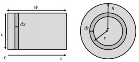
In order to model the two-dimensional object (the plane), we model it has being the sum of many one dimensional objects. We can model a plane either as a rectangle of width, $W$, and length, $L$, as shown in the left panel of Figure $\PageIndex{10}$ or as a disk of radius, $R$, as shown in the right panel. To model an infinite plane, we can then take the limit of either $L$ and $W$ going to infinity (rectangle), or of $R$ going to infinity (disk). We can model the rectangle as being the sum of many lines of finite length, $L$, and infinitesimal width, $dx$. Similarly, we can model the disk as the sum of infinitesimally thin rings of finite radius, $r$, and thickness, $dr$. In both cases, we know how to model the field from a line of charge (Example 16.3.3) or from a ring (Example 16.3.2).

Figure $\PageIndex{10}$: A two-dimensional object such as a plane modeled as a sum of infinitely thin lines (left panel) or as the sum of infinitely thin rings (right panel).

We proceed by modeling the plane as a disk made up of infinitesimal rings. Our infinitesimal charge, $dq$, is thus the charge on a ring of radius $r$ and thickness $dr$, as illustrated in Figure $\PageIndex{11}$.

Figure $\PageIndex{11}$: Modeling the field from a disk as the sum of fields from concentric thin rings.

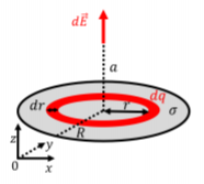
We know from Example 16.3.2 that the magnitude of the electric field a distance $a$ from the center of the ring, along its axis of symmetry (the $z$ axis in Figure $\PageIndex{11}$), is given by:

$$\begin{aligned} dE = kdq\frac{a}{(r^2+a^2)^\frac{3}{2}} \end{aligned}$$

By symmetry, for all of the different infinitesimal rings that make up the disk, the field will always point along the $z$ axis. In order to determine the total field, we sum (integrate) the values of $dE$, over all of the rings, from a radius of $r=0$ to a radius $r=R$. For each ring, the value of $r$ will be different, so we need to express $dq$ in terms of $dr$ in order to perform the integral. We know that the plane has a uniform charge per unit area given by $\sigma$. The charge $dq$ of an infinitesimal ring is given by:

$$\begin{aligned} dq = \sigma dA=\sigma 2\pi r dr\end{aligned}$$

where $dA=2\pi r dr$ is the area of the infinitesimal ring of radius $r$ and thickness $dr$ (think of unfolding the ring into a rectangle of height $dr$ and length $2\pi r$, the circumference of the circle, in order to determine the area). We now have all of the ingredients in order to determine the total electric field:

$$\begin{aligned} E &= \int dE = \int_0^R kdq\frac{a}{(r^2+a^2)^\frac{3}{2}} = 2\pi k a \sigma \int_0^R \frac{r}{(r^2+a^2)^\frac{3}{2}}dr\\[4pt] &=2\pi k a \sigma \left[ \frac{-1}{\sqrt{r^2+a^2}}\right]_0^R=2\pi k \sigma\left(1-\frac{a}{R^2+a^2} \right)\end{aligned}$$

Finally, we can take the limit of $R\to\infty$ in order to get the electric field above an infinite plane:

$$\begin{aligned} E=\lim_{R\to\infty}2\pi k \sigma\left(1-\frac{a}{R^2+a^2} \right)=2\pi k\sigma=\frac{\sigma}{2\epsilon_0}\end{aligned}$$

where we used $\epsilon_0$ in the last equality as the result is a little cleaner without the factors of $\pi$. Note that for an infinite plane of charge, the electric field does not depend on the distance (our variable $a$) from the plane!

Discussion

In this example, we showed how we can model a two-dimensional charge distribution as the sum of one-dimensional charge distributions. In particular, we showed that an infinite plane of charge can be modeled as the sum of many lines charges or of many rings of charge (we chose the latter in the above). We also found that the electric field above an infinite plane of charge does not depend on the distance from the plane; that is, the electric field is constant above an infinite plane of charge.

josh's thoughts

A common source of confusion is the process of solving for the electric field produced by continuous charges. Point charges are well defined in space as being entirely contained within a single point, while continuous charges are objects which occupy 1, 2, or 3 dimensions. The electric field produced by point charges are easily modeled by $\vec E = \frac{kQ}{r^2}\hat r$, but the electric fields produced by continuous charges must usually be obtained from an integral.

When a charge is distributed, the charge on the object must be broken down into many small charges which are written as $dq$. From there, $dq$ is rewritten in terms of a position variable over which it is convenient to integrate. Think of the position variable as a variable that you can use to distinguish charges, $dq$, located at different positions along the object.

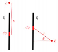
For example, referring to Figure $\PageIndex{12}$, if I wanted to determine $E$ at the top of a rod (left-hand panel), it would be most convenient for me to integrate over $x$, but if I wanted to determine $E$ on the side of a rod, it would be most convenient to integrate over $\theta$.

Figure $\PageIndex{12}$: Calculating the electric field produced by a rod at different positions.

In order to determine the bounds of the integral, think of the range in position variable that is required in order to cover the entire object. I recommend paying close attention to Examples 16.3.2, 16.3.3, and 16.3.4, and attempting questions which require integration on the Question Library.