22.7: Sample problems and solutions

Exercise \(\PageIndex{1}\)

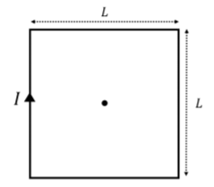
A square loop of wire with side length, \(L\), carries current, \(I\), as shown in Figure \(\PageIndex{1}\). What is the magnetic field at the center of the loop?

Figure \(\PageIndex{1}\): A square loop of current.

Answer

The square loop is simply made of four straight sections of wire of length, \(L\). The magnetic field from each section of wire is into the page, which you can easily verify with your right-hand (with your thumb in the direction of current, your fingers curl in the direction of the resulting magnetic field).

The magnetic field at the center is just four times the magnetic field produced by a single segment, which we determined in this chapter. The magnetic field at the center of the loop is thus four times the magnetic field at a distance, \(h = \frac{L}{2}\), from a wire of length, \(L\):

\[\begin{aligned} B=4\times\frac{\mu_{0}I}{2\pi\frac{L}{2}}\frac{L/2}{\sqrt{\frac{L^{2}}{4}+\frac{L^{2}}{4}}}=2\sqrt{2}\frac{\mu_{0}I}{\pi L} \end{aligned}\]

Exercise \(\PageIndex{2}\)

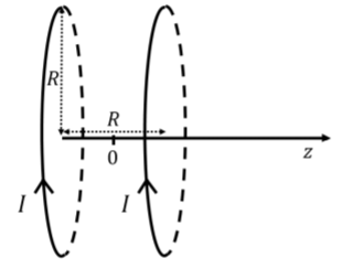
Helmholtz coils are an arrangement of two parallel loops of current which produce a nearly uniform magnetic field. Helmholtz coils are formed by two identical circular loops of radius, \(R\), carrying the same current, \(I\), where the centers of the coils are separated by the distance, \(R\), as illustrated in Figure \(\PageIndex{2}\). Determine the magnetic field as a function of \(z\), along the axis of symmetry of the coils, where the origin is located half way between the two coils. Make a plot of the magnetic field as a function of \(z\) from each coil, as well as the total electric field to show that it is close to uniform between the coils.

Figure \(\PageIndex{2}\): A Helmholtz coil arrangement.

Answer

We know that the magnetic field at a distance, \(h\), from the center of a loop of current, along its axis of symmetry is given by:

\[\begin{aligned} B(h)=\frac{\mu_{0}I}{2}\frac{R^{2}}{(R^{2}+h^{2})^{\frac{3}{2}}} \end{aligned}\]

For the two coils in the Helmholtz configuration, the magnetic field from each coil will be in the same direction. The center of the two coils are located at \(z = ±\frac{R}{2}\). Thus, if we are located at position, \(z\), along the \(z\) axis, one coil will be at a distance of \(z +\frac{R}{2}\), and the other at a distance \(z −\frac{R}{2}\). The total magnetic field as a function of \(z\) is then given by:

\[\begin{aligned} B^{tot}(z)&=B\left(z+\frac{R}{2}\right)+B\left(z+\frac{R}{2}\right) \\[4pt] &= \frac{\mu_{0}I}{2}\frac{R^{2}}{(R^{2}+(z+\frac{R}{2})^{2})^{\frac{3}{2}}}+\frac{\mu_{0}I}{2}\frac{R^{2}}{(R^{2}+(z-\frac{R}{2})^{2})^{\frac{3}{2}}} \end{aligned}\]

We can plot this function, as well as the two individual terms using python. For information, we show the code below. In order to make the plot, we need to choose some reasonable values for the radius of the coils and the current through the coils, for example:

• \(R=0.3\text{m}\)
• \(I=0.1\text{A}\)

Python Code 22.7.1: Numerical integration of a function

#Import the modules that we need:
import numpy as np
import pylab as pl

#Define some constants:
mu0 = 4*np.pi*1e-7 #4 pi
I = 0.5
R = 0.3

#Define the values on the z axis, from -2R to +2r, in 100 increments
z = np.linspace(-2*R,2*R,100)

#Determine the magnetic field from the coils at those values of z
#The coil at z=-R/2:
B1 = (mu0*I)/2 * R**2/((R**2+(z+R/2)**2)**(3/2))
#The coil at z=+R/2:
B2 = (mu0*I)/2 * R**2/((R**2+(z-R/2)**2)**(3/2))
#The sum:
B = B1 + B2

#Make the plot
p1.figure(figsize=(10,6))
p1.plot(z,B1,label='Coil at z=-R/2')
p1.plot(z,B2,label='Coil at z=+R/2')
p1.plot(z,B,label='Total')
p1.legend()
p1.xlabel('z position [m]')
p1.ylabel('Magnetic field [T]')
p1.show()

Output 22.7.1:

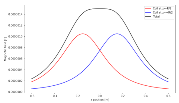
Figure \(\PageIndex{3}\): Magnetic field from each coil, as well as their sum, for two coils in the Helmholtz configuration.

As advertised, we see a region between the Helmholtz coils where the magnetic field is nearly uniform.