3.6: Electric Field Lines

Learning Objectives

By the end of this section, you will be able to:

• Calculate the total force (magnitude and direction) exerted on a test charge from more than one charge
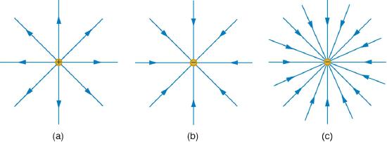
• Describe an electric field diagram of a positive point charge; of a negative point charge with twice the magnitude of positive charge
• Draw the electric field lines between two points of the same charge; between two points of opposite charge.

Drawings using lines to represent electric fields around charged objects are very useful in visualizing field strength and direction. Since the electric field has both magnitude and direction, it is a vector. Like all vectors, the electric field can be represented by an arrow that has length proportional to its magnitude and that points in the correct direction. (We have used arrows extensively to represent force vectors, for example.)

Figure \(\PageIndex{1}\) shows two pictorial representations of the same electric field created by a positive point charge \(Q\). Figure \(\PageIndex{1}\) (b) shows the standard representation using continuous lines. Figure \(\PageIndex{1}\) (b) shows numerous individual arrows with each arrow representing the force on a test charge \(q\). Field lines are essentially a map of infinitesimal force vectors.

Figure \(\PageIndex{1}\): Two equivalent representations of the electric field due to a positive charge \(Q\). (a) Arrows representing the electric field’s magnitude and direction. (b) In the standard representation, the arrows are replaced by continuous field lines having the same direction at any point as the electric field. The closeness of the lines is directly related to the strength of the electric field. A test charge placed anywhere will feel a force in the direction of the field line; this force will have a strength proportional to the density of the lines (being greater near the charge, for example).

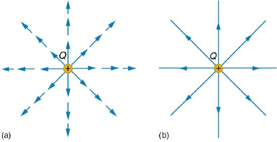
Note that the electric field is defined for a positive test charge \(q\), so that the field lines point away from a positive charge and toward a negative charge. (Figure \(\PageIndex{2}\)) The electric field strength is exactly proportional to the number of field lines per unit area, since the magnitude of the electric field for a point charge is \(E=k|Q|/r^{2}\) and area is proportional to \(r^{2}\). This pictorial representation, in which field lines represent the direction and their closeness (that is, their areal density or the number of lines crossing a unit area) represents strength, is used for all fields: electrostatic, gravitational, magnetic, and others.

Figure \(\PageIndex{2}\): The electric field surrounding three different point charges. (a) A positive charge. (b) A negative charge of equal magnitude. (c) A larger negative charge.

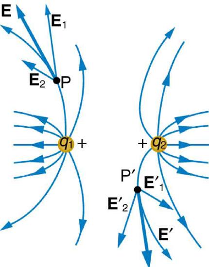
In many situations, there are multiple charges. The total electric field created by multiple charges is the vector sum of the individual fields created by each charge. Figure \(\PageIndex{4}\) shows how the electric field from two point charges can be drawn by finding the total field at representative points and drawing electric field lines consistent with those points. While the electric fields from multiple charges are more complex than those of single charges, some simple features are easily noticed.

Figure \(\PageIndex{4}\): Two positive point charges \(q_{1}\) and \(q_{2}\) produce the resultant electric field shown. The field is calculated at representative points and then smooth field lines drawn following the rules outlined in the text.

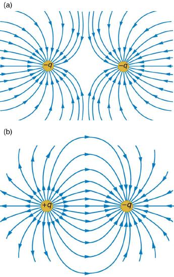
For example, the field is weaker between like charges, as shown by the lines being farther apart in that region. (This is because the fields from each charge exert opposing forces on any charge placed between them.) (See Figure \(\PageIndex{4}\) and Figure \(\PageIndex{5}\)(a).) Furthermore, at a great distance from two like charges, the field becomes identical to the field from a single, larger charge.

Figure \(\PageIndex{5}\)(b) shows the electric field of two unlike charges. The field is stronger between the charges. In that region, the fields from each charge are in the same direction, and so their strengths add. The field of two unlike charges is weak at large distances, because the fields of the individual charges are in opposite directions and so their strengths subtract. At very large distances, the field of two unlike charges looks like that of a smaller single charge.

Figure \(\PageIndex{5}\): (a) Two negative charges produce the fields shown. It is very similar to the field produced by two positive charges, except that the directions are reversed. The field is clearly weaker between the charges. The individual forces on a test charge in that region are in opposite directions. (b) Two opposite charges produce the field shown, which is stronger in the region between the charges.

We use electric field lines to visualize and analyze electric fields (the lines are a pictorial tool, not a physical entity in themselves). The properties of electric field lines for any charge distribution can be summarized as follows:

1. Field lines must begin on positive charges and terminate on negative charges, or at infinity in the hypothetical case of isolated charges.
2. The number of field lines leaving a positive charge or entering a negative charge is proportional to the magnitude of the charge.
3. The strength of the field is proportional to the closeness of the field lines—more precisely, it is proportional to the number of lines per unit area perpendicular to the lines.
4. The direction of the electric field is tangent to the field line at any point in space.
5. Field lines can never cross.

The last property means that the field is unique at any point. The field line represents the direction of the field; so if they crossed, the field would have two directions at that location (an impossibility if the field is unique).

Summary

• Drawings of electric field lines are useful visual tools. The properties of electric field lines for any charge distribution are that:
• Field lines must begin on positive charges and terminate on negative charges, or at infinity in the hypothetical case of isolated charges.
• The number of field lines leaving a positive charge or entering a negative charge is proportional to the magnitude of the charge.
• The strength of the field is proportional to the closeness of the field lines—more precisely, it is proportional to the number of lines per unit area perpendicular to the lines.
• The direction of the electric field is tangent to the field line at any point in space.
• Field lines can never cross.

Glossary

electric field

a three-dimensional map of the electric force extended out into space from a point charge

electric field lines

a series of lines drawn from a point charge representing the magnitude and direction of force exerted by that charge

vector

a quantity with both magnitude and direction

vector addition

mathematical combination of two or more vectors, including their magnitudes, directions, and positions