4.2: Electric Potential Energy and Electrical Potential Difference

Learning Objectives

By the end of this section, you will be able to:

• Define electric potential and electric potential energy.
• Describe the relationship between potential difference and electrical potential energy.
• Explain electron volt and its usage in submicroscopic process.
• Determine electric potential energy given potential difference and amount of charge.

Electrical Potential Energy

When a free positive charge \(q\) is accelerated by an electric field, such as shown in Figure \(\PageIndex{1}\), it is given kinetic energy. The process is analogous to an object being accelerated by a gravitational field. It is as if the charge is going down an electrical hill where its electric potential energy is converted to kinetic energy. Let us explore the work done on a charge \(q\) by the electric field in this process, so that we may develop a definition of electric potential energy.

Figure \(\PageIndex{1}\): A charge accelerated by an electric field is analogous to a mass going down a hill. In both cases potential energy is converted to another form. Work is done by a force, but since this force is conservative, we can write \(W=-\Delta \mathrm{PE}\).

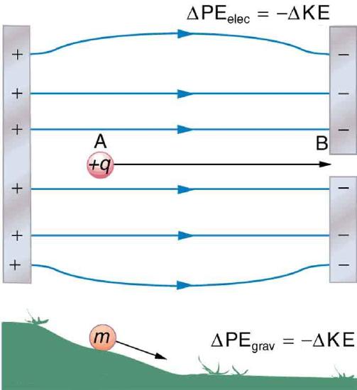
The electrostatic or Coulomb force is conservative, which means that the work done on \(q\) is independent of the path taken. This is exactly analogous to the gravitational force in the absence of dissipative forces such as friction. When a force is conservative, it is possible to define a potential energy associated with the force, and it is usually easier to deal with the potential energy (because it depends only on position) than to calculate the work directly.

We use U to denote electric potential energy, which has units of joules (J). The change in potential energy, \(\Delta \mathrm{U}\), is crucial, since the work done by a conservative force is the negative of the change in potential energy; that is, \(W=-\Delta \mathrm{U}\). For example, work \(W\) done to accelerate a positive charge from rest is positive and results from a loss in U, or a negative \(\Delta \mathrm{U}\). There must be a minus sign in front of \(\Delta \mathrm{U}\) to make \(W\) positive. U can be found at any point by taking one point as a reference and calculating the work needed to move a charge to the other point.

ELECTRICAL POTENTIAL ENERGY

\(W=-\Delta \mathrm{U}\). For example, work \(W\) done to accelerate a positive charge from rest is positive and results from a loss in U, or a negative \(\Delta \mathrm{U}\) There must be a minus sign in front of \(\Delta \mathrm{U}\) to make \(W\) positive. U can be found at any point by taking one point as a reference and calculating the work needed to move a charge to the other point.

Gravitational potential energy and electric potential energy are quite analogous. Potential energy accounts for work done by a conservative force and gives added insight regarding energy and energy transformation without the necessity of dealing with the force directly. It is much more common, for example, to use the concept of voltage (related to electric potential energy) than to deal with the Coulomb force directly.

Calculating the work directly is generally difficult, since \(W=Fd\cos \theta\) and the direction and magnitude of \(F\) can be complex for multiple charges, for odd-shaped objects, and along arbitrary paths. But we do know that, since \(F=qE\), the work, and hence \(\Delta \mathrm{U}\), is proportional to the test charge \(q\) To have a physical quantity that is independent of test charge, we define electric potential \(V\) (or simply potential, since electric is understood) to be the potential energy per unit charge:

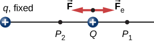
To show this explicitly, consider an electric charge \(+q\) fixed at the origin and move another charge \(+Q\) toward q in such a manner that, at each instant, the applied force \(\vec{F}\) exactly balances the electric force \(\vec{F}_e\) on Q (Figure \(\PageIndex{2}\)). The work done by the applied force \(\vec{F}\) on the charge Q changes the potential energy of Q. We call this potential energy the electrical potential energy of Q.

Figure \(\PageIndex{2}\): Displacement of “test” charge Q in the presence of fixed “source” charge q.

The work \(W_{12}\) done by the applied force \(\vec{F}\) when the particle moves from \(P_1\) to \(P_2\) may be calculated by

\[W_{12} = \int_{P_1}^{P_2} \vec{F} \cdot d\vec{l}.\]

Since the applied force \(\vec{F}\) balances the electric force \(\vec{F}_e\) on Q, the two forces have equal magnitude and opposite directions. Therefore, the applied force is

\[\vec{F} = -\vec{F}_e = - \dfrac{kqQ}{r^2} \hat{r},\]

where we have defined positive to be pointing away from the origin and r is the distance from the origin. The directions of both the displacement and the applied force in the system in Figure \(\PageIndex{2}\) are parallel, and thus the work done on the system is positive.

We use the letter U to denote electric potential energy, which has units of joules (J). When a conservative force does negative work, the system gains potential energy. When a conservative force does positive work, the system loses potential energy, \(\Delta U = - W\). In the system in Figure \(\PageIndex{3}\), the Coulomb force acts in the opposite direction to the displacement; therefore, the work is negative. However, we have increased the potential energy in the two-charge system.

Example \(\PageIndex{1}\): Kinetic Energy of a Charged Particle

A \(+3.0-nC\) charge Q is initially at rest a distance of 10 cm (\(r_1\)) from a \(+5.0-nC\) charge q fixed at the origin (Figure \(\PageIndex{3}\)). Naturally, the Coulomb force accelerates Q away from q, eventually reaching 15 cm (\(r_2\)).

Figure \(\PageIndex{3}\): The charge Q is repelled by q, thus having work done on it and gaining kinetic energy.

1. What is the work done by the electric field between \(r_1\) and \(r_2\)?
2. How much kinetic energy does Q have at \(r_2\)?

Strategy

Calculate the work with the usual definition. Since Q started from rest, this is the same as the kinetic energy.

Solution

Integrating force over distance, we obtain

\[\begin{align} W_{12} &= \int_{r_1}^{r_2} \vec{F} \cdot d\vec{r} \nonumber \\[4pt] &= \int_{r_1}^{r_2} \dfrac{kqQ}{r^2}dr \nonumber \\[4pt] &= \left. - \dfrac{kqQ}{r} \right|_{r_1}^{r_2} \nonumber \\[4pt] &= kqQ \left[\dfrac{-1}{r_2} + \dfrac{1}{r_1}\right] \nonumber \\[4pt] &= (8.99 \times 10^9 \, Nm^2/C^2)(5.0 \times 10^{-9} C)(3.0 \times 10^{-9} C) \left[ \dfrac{-1}{0.15 \, m} + \dfrac{1}{0.10 \, m}\right] \nonumber \\[4pt] &= 4.5 \times 10^{-7} \, J. \nonumber \end{align} \nonumber\]

This is also the value of the kinetic energy at \(r_2\).

Significance

Charge Q was initially at rest; the electric field of q did work on Q, so now Q has kinetic energy equal to the work done by the electric field.

 In this example, the work W done to accelerate a positive charge from rest is positive and results from a loss in U, or a negative \(\Delta U\). A value for U can be found at any point by taking one point as a reference and calculating the work needed to move a charge to the other point.

Electric Potential Energy

Work W done to accelerate a positive charge from rest is positive and results from a loss in U, or a negative \(\Delta U\). Mathematically,

\[W = - \Delta U. \label{7.1}\]

Gravitational potential energy and electric potential energy are quite analogous. Potential energy accounts for work done by a conservative force and gives added insight regarding energy and energy transformation without the necessity of dealing with the force directly. It is much more common, for example, to use the concept of electric potential energy than to deal with the Coulomb force directly in real-world applications.

In polar coordinates with q at the origin and Q located at r, the displacement element vector is \(d\vec{l} = \hat{r} dr\) and thus the work becomes

\[\begin{align} W_{12} &= kqQ \int_{r_1}^{r_2} \dfrac{1}{r^2} \hat{r} \cdot \hat{r} dr \nonumber \\[4pt] &= \underbrace{kqQ \dfrac{1}{r_2}}_{final \, point} - \underbrace{kqQ \dfrac{1}{r_1}}_{initial \,point}. \end{align}\]

Notice that this result only depends on the endpoints and is otherwise independent of the path taken. To explore this further, compare path \(P_1\) to \(P_2\) with path \(P_1 P_3 P_4 P_2\) in Figure \(\PageIndex{4}\).

Figure \(\PageIndex{4}\):Two paths for displacement \(P_1\) to \(P_2\). The work on segments \(P_1P_3\) and \(P_4P_2\) are zero due to the electrical force being perpendicular to the displacement along these paths. Therefore, work on paths \(P_1P_2\) and \(P_1P_3P_4P_2\) are equal.

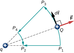
The segments \(P_1P_3\) and \(P_4P_2\) are arcs of circles centered at q. Since the force on Q points either toward or away from q, no work is done by a force balancing the electric force, because it is perpendicular to the displacement along these arcs. Therefore, the only work done is along segment \(P_3P_4\) which is identical to \(P_1P_2\).

One implication of this work calculation is that if we were to go around the path \(P_1P_3P_4P_2P_1\), the net work would be zero (Figure \(\PageIndex{5}\)). Recall that this is how we determine whether a force is conservative or not. Hence, because the electric force is related to the electric field by \(\vec{F} = g\vec{E}\), the electric field is itself conservative.

Figure \(\PageIndex{5}\): A closed path in an electric field. The net work around this path is zero.

Another implication is that we may define an electric potential energy. Recall that the work done by a conservative force is also expressed as the difference in the potential energy corresponding to that force. Therefore, the work \(W_{ref}\) to bring a charge from a reference point to a point of interest may be written as

\[W_{ref} = \int_{r_{ref}}^r \vec{F} \cdot d\vec{l}\]

and, by Equation \ref{7.1}, the difference in potential energy (\(U_2 - U_1\)) of the test charge Q between the two points is

\[\Delta U = - \int_{r_{ref}}^r \vec{F} \cdot d\vec{l}.\]

Therefore, we can write a general expression for the potential energy of two point charges (in spherical coordinates):

\[\Delta U = - \int_{r_{ref}}^r \dfrac{kqQ}{r^2}dr = -\left[-\dfrac{kqQ}{r}\right]_{r_{ref}}^r = kqQ\left[ \dfrac{1}{r} - \dfrac{1}{r_{ref}}\right].\]

We may take the second term to be an arbitrary constant reference level, which serves as the zero reference:

\[U(r) = k\dfrac{qQ}{r} - U_{ref}.\]

A convenient choice of reference that relies on our common sense is that when the two charges are infinitely far apart, there is no interaction between them. (Recall the discussion of reference potential energy in Potential Energy and Conservation of Energy.) Taking the potential energy of this state to be zero removes the term \(U_{ref}\) from the equation (just like when we say the ground is zero potential energy in a gravitational potential energy problem), and the potential energy of Q when it is separated from q by a distance r assumes the form

\[\underbrace{U(r) = k\dfrac{qQ}{r}}_{zero \, reference \, at \, r = \infty}.\]

This formula is symmetrical with respect to \(q\) and \(Q\), so it is best described as the potential energy of the two-charge system.

Example \(\PageIndex{2}\): Potential Energy of a Charged Particle

A \(+3.0-nC\) charge Q is initially at rest a distance of 10 cm \((r_1)\) from a \(+5.0-nC\) charge q fixed at the origin (Figure \(\PageIndex{6}\)). Naturally, the Coulomb force accelerates Q away from q, eventually reaching 15 cm \((r_2)\).

Figure \(\PageIndex{6}\): The charge \(Q\) is repelled by \(q\), thus having work done on it and losing potential energy.

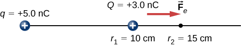
What is the change in the potential energy of the two-charge system from \(r_1\) to \(r_2\)?

Strategy

Calculate the potential energy with the definition given above:

\(\Delta U_{12} = -\int_{r_1}^{r_2} \vec{F} \cdot d\vec{r}\). Since Q started from rest, this is the same as the kinetic energy.

Solution

We have

\[\begin{align} \Delta U_{12} &= - \int_{r_1}^{r_2} \vec{F} \cdot d\vec{r} \nonumber \\[4pt] &= - \int_{r_1}^{r_2} \dfrac{kqQ}{r^2}dr \nonumber \\[4pt] &= - \left[ - \dfrac{kqQ}{r}\right]_{r_1}^{r_2} \nonumber \\[4pt] &=kqQ \left[ \dfrac{1}{r_2} - \dfrac{1}{r_1} \right] \nonumber \\[4pt] &= (8.99 \times 10^9 \, Nm^2/C^2)(5.0 \times 10^{-9} C)(3.0 \times 10^{-9} C) \left[ \dfrac{1}{0.15 \, m} - \dfrac{1}{0.10 \, m}\right] \nonumber \\[4pt] &= - 4.5 \times 10^{-7} \, J. \end{align} \]

Significance

The change in the potential energy is negative, as expected, and equal in magnitude to the change in kinetic energy in this system. Recall from Example \(\PageIndex{1}\) that the change in kinetic energy was positive.

Due to Coulomb’s law, the forces due to multiple charges on a test charge \(Q\) superimpose; they may be calculated individually and then added. This implies that the work integrals and hence the resulting potential energies exhibit the same behavior. To demonstrate this, we consider an example of assembling a system of four charges.

Example \(\PageIndex{3}\): Assembling Four Positive Charges

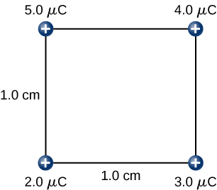
Find the amount of work an external agent must do in assembling four charges \(+2.0-\mu C\), \(+3.0-\mu C\), \(+4.0-\mu C\) and \(+5.0-\mu C\) at the vertices of a square of side 1.0 cm, starting each charge from infinity (Figure \(\PageIndex{7}\)).

Figure \(\PageIndex{7}\): How much work is needed to assemble this charge configuration?

Strategy

We bring in the charges one at a time, giving them starting locations at infinity and calculating the work to bring them in from infinity to their final location. We do this in order of increasing charge.

Solution

Step 1. First bring the \(+2.0-\mu C\) charge to the origin. Since there are no other charges at a finite distance from this charge yet, no work is done in bringing it from infinity,

\[W_1 = 0.\]

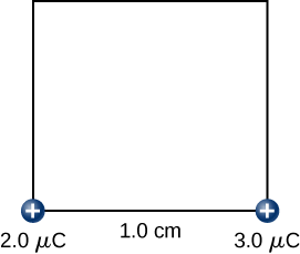
Step 2. While keeping the \(+2.0-\mu C\) charge fixed at the origin, bring the \(+3.0-\mu C\) charge to \((x,y,z) = (1.0 \, cm, \, 0, \, 0)\) (Figure \(\PageIndex{8}\)). Now, the applied force must do work against the force exerted by the \(+2.0-\mu C\) charge fixed at the origin. The work done equals the change in the potential energy of the \(+3.0-\mu C\) charge:

\[\begin{align} W_2 &= k\dfrac{q_1q_2}{r{12}} \nonumber \\[4pt] &= \left(9.0 \times 10^9 \frac{N \cdot m^2}{C^2}\right) \dfrac{(2.0 \times 10^{-6} C)(3.0 \times 10^{-6}C)}{1.0 \times 10^{-2} m} \nonumber \\[4pt] &= 5.4 \, J.\nonumber \end{align} \nonumber\]

Figure \(\PageIndex{8}\): Step 2. Work \(W_2\) to bring the \(+3.0-\mu C\) charge from infinity.

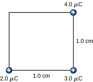
Step 3. While keeping the charges of \(+2.0-\mu C\) and \(+3.0-\mu C\) fixed in their places, bring in the \(+4.0-\mu C\) charge to \((x,y,z) = (1.0 \, cm, \, 1.0 \, cm, \, 0)\) (Figure)\(\PageIndex{9}\). The work done in this step is

\[\begin{align} W_3 &= k\dfrac{q_1q_3}{r_{13}} + k \dfrac{q_2q_3}{r_{23}} \nonumber \\[4pt] &= \left(9.0 \times 10^9 \frac{N \cdot m^2}{C^2}\right) \left[ \dfrac{(2.0 \times 10^{-6}C)(4.0 \times 10^{-6}C)}{\sqrt{2} \times 10^{-2}m} + \dfrac{(3.0 \times 10^{-6} C)(4.0 \times 10^{-6}C)}{1.0 \times 10^{-2} m}\right] \nonumber \\[4pt] &= 15.9 \, J. \nonumber \end{align} \nonumber\]

Figure \(\PageIndex{9}\): Step 3. The work \(W_3\) to bring the \(+4.0-\mu C\) charge from infinity.

Step 4. Finally, while keeping the first three charges in their places, bring the \(+5.0-\mu C\) charge to \((x,y,z) = (0, \, 1.0 \, cm, \, 0)\) (Figure \(\PageIndex{10}\)). The work done here is

\[\begin{align} W_4 &= kq_4 \left[ \dfrac{q_1}{r_{14}} + \dfrac{q_2}{r_{24}} + \dfrac{q_3}{r_{34}}\right], \nonumber \\[4pt] &= \left(9.0 \times 10^9 \frac{N \cdot m^2}{C^2}\right)(5.0 \times 10^{-6}C) \left[ \dfrac{(2.0 \times 10^{-6}C)}{1.0 \times 10^{-2}m} + \dfrac{(3.0 \times 10^{-6} C)} {\sqrt{2} \times 10^{-2} m} + \dfrac{(4.0 \times 10^{-6}C)}{1.0 \times 10^{-2}m} \right] \nonumber \\[4pt] &= 36.5 \, J. \nonumber \end{align} \nonumber\]

Figure \(\PageIndex{10}\): Step 4. The work \(W_4\) to bring the \(+5.0-\mu C\) charge from infinity.

Hence, the total work done by the applied force in assembling the four charges is equal to the sum of the work in bringing each charge from infinity to its final position:

\[\begin{align} W_T &= W_1 + W_2 + W_3 + W_4 \nonumber \\[4pt] &= 0 + 5.4 \, J + 15.9 \, J + 36.5 \, J \nonumber \\[4pt] &= 57.8 \, J. \nonumber \end{align} \nonumber\]

Significance

The work on each charge depends only on its pairwise interactions with the other charges. No more complicated interactions need to be considered; the work on the third charge only depends on its interaction with the first and second charges, the interaction between the first and second charge does not affect the third.

positive, negative, and these quantities are the same as the work you would need to do to bring the charges in from infinity

Note that the electrical potential energy is positive if the two charges are of the same type, either positive or negative, and negative if the two charges are of opposite types. This makes sense if you think of the change in the potential energy \(\Delta U\) as you bring the two charges closer or move them farther apart. Depending on the relative types of charges, you may have to work on the system or the system would do work on you, that is, your work is either positive or negative. If you have to do positive work on the system (actually push the charges closer), then the energy of the system should increase. If you bring two positive charges or two negative charges closer, you have to do positive work on the system, which raises their potential energy. Since potential energy is proportional to 1/r, the potential energy goes up when r goes down between two positive or two negative charges.

On the other hand, if you bring a positive and a negative charge nearer, you have to do negative work on the system (the charges are pulling you), which means that you take energy away from the system. This reduces the potential energy. Since potential energy is negative in the case of a positive and a negative charge pair, the increase in 1/r makes the potential energy more negative, which is the same as a reduction in potential energy.

The result from Example \(\PageIndex{2}\) may be extended to systems with any arbitrary number of charges. In this case, it is most convenient to write the formula as

\[W_{12 . . . N} = \dfrac{k}{2} \sum_i^N \sum_j^N \dfrac{q_iq_j}{r_{ij}} \, for \, i \neq j.\]

The factor of 1/2 accounts for adding each pair of charges twice.

 

Consider two point charges, \(q_1\) and \(q_2\) that are separated by an initial distance \(r_A\) and are moved to a new separation \(r_B\) (we will assume that only \(q_2\) moves). We seek the work done on \(q_2\) during this move by the electric field coming from \(q_1\), from which we can obtain the change in the system's potential energy.

Figure 2.1.1 – Change of Potential Energy for a Two Point Charges

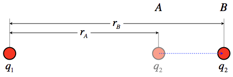
The force between these charges changes as \(q_2\) is moved, which means that the work calculation requires a far less trivial integral than was performed for the case of a uniform field. Start by setting up the work integral with the coluomb force:

\[\overrightarrow F_{on\;q_2} = \dfrac{q_1q_2}{4\pi\epsilon_or^2}\widehat r \;\;\; \Rightarrow \;\;\; W_{A\rightarrow B}=\int\limits_A^B \overrightarrow F\cdot\overrightarrow{dl} = \int\limits_A^B \left(\dfrac{q_1q_2}{4\pi\epsilon_or^2}\widehat r\right)\cdot\overrightarrow{dl}\]

The displacement is parallel to the radial unit vector (if it wasn't, the dot product would require that we only take the displacement in that direction anyway), so the product \(\widehat r \cdot \overrightarrow{dl}\) can be written simply as \(+dr\). Putting this into the integral gives:

\[W_{A\rightarrow B}=\dfrac{q_1q_2}{4\pi\epsilon_o}\int\limits_{r_A}^{r_B} \dfrac{1}{r^2}dr = \dfrac{q_1q_2}{4\pi\epsilon_o}\left[ \dfrac{1}{r_A}-\dfrac{1}{r_B}\right]\]

The change in potential energy for this process is therefore:

\[\Delta U = -W_{A\rightarrow B} = \dfrac{q_1q_2}{4\pi\epsilon_o}\left[ \dfrac{1}{r_B}-\dfrac{1}{r_A}\right]\]

As we recall from our study of mechanics, it is only the change in potential energy that matters, but we also find it useful to define a state of zero potential, from which we can reference other states. It is common (though not universal, as well will see later) to reference our point of zero electrostatic potential energy at \(r=\infty\). Another way to look at this is to think of the potential energy of a configuration of charges (in this case, two point charges) as the work done in moving the charges from infinite separation to their current proximity. That gives us the following potential energy of two point charges separated by a distance \(r\):

\[U\left(r\right) = -W_{\infty\rightarrow r} = \dfrac{q_1q_2}{4\pi\epsilon_or}\]

It should be noted that this potential energy is positive if the two charges have the same sign, and negative if they have different signs. This makes sense, since we have to add external work to the system to push the repelling charges together, while attracting charges "want" to come together, which is a characteristic of decreasing potential energy (because the force causes them to speed up, so the loss of potential energy results in a increase of kinetic energy).

When we collect more than just two point charges, we have to account for the potential energy contribution of every pair of charges. This begins to add up when the number of point charges grows. Representing the separation of charge 1 from charge 2 with "\(r_{12}\)", charge 1 from charge 3 with "\(r_{13}\)," and so on, the total potential energy for a collection of point charges is the sum of all the pairwise contributions:

\[U_{total} = \dfrac{q_1q_2}{4\pi\epsilon_or_{12}}+\dfrac{q_1q_3}{4\pi\epsilon_or_{13}}+\dfrac{q_2q_3}{4\pi\epsilon_or_{23}}\dots\]

Example \(\PageIndex{4}\)

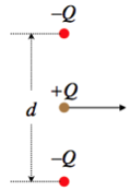
A point charge \(Q\) is moving horizontally halfway between two other point charges that are equal in magnitude but opposite in sign, and are held fixed in place. The two negative point charges are separated by a distance \(d\). The positive point charge obviously experiences no net vertical force, so it continues moving horizontally. Find the amount of KE gained or lost (indicate which) by the moving charge at the moment when the three charges form an equilateral triangle.

Solution

The mechanical energy will be conserved, so the change in kinetic energy will equal the negative the change of potential energy. The potential energy in the system that results from the two negative charges interacting with each other never changes (they are held in place), and the potential energy change between the moving charge each of the stationary charges is the same due to symmetry. So all we need to calculate is the change in potential energy between the moving charge and one of the others, and multiply it by two. They are initially separated by a distance \(\frac{d}{2}\), and afterward are separated by \(d\), so:

\[\Delta KE=-\Delta U_{system} = -2\left[\dfrac{-Q^2}{4\pi\epsilon_od}-\dfrac{-Q^2}{4\pi\epsilon_o\frac{d}{2}}\right]=-\dfrac{Q^2}{2\pi\epsilon_od}\nonumber\]

The change in kinetic energy is negative, indicating that the charge slows down. This makes sense, given that it is attracted by the other charges, which pull it in the direction opposite to its motion.

 

Electrical Potential 

Calculating the work directly is generally difficult, since \(W=Fd\cos \theta\) and the direction and magnitude of \(F\) can be complex for multiple charges, for odd-shaped objects, and along arbitrary paths. But we do know that, since \(F=qE\), the work, and hence \(\Delta \mathrm{U}\), is proportional to the test charge \(q\) To have a physical quantity that is independent of test charge, we define electric potential \(V\) (or simply potential, since electric is understood) to be the potential energy per unit charge:

\[V=\dfrac{\mathrm{U}}{q}.\]

ELECTRIC POTENTIAL

This is the electric potential energy per unit charge.

\[V=\dfrac{\mathrm{U}}{q}\]

Since PE is proportional to \(q\), the dependence on \(q\) cancels. Thus \(V\) does not depend on \(q\). The change in potential energy \(\Delta \mathrm{U}\) is crucial, and so we are concerned with the difference in potential or potential difference \(\Delta V\) between two points, where

\[\Delta V =V_{B}-V_{A}=\dfrac{\Delta \mathrm{U}}{q}.\]

The potential difference between points A and B, \(V_{B}-V_{A}\), is thus defined to be the change in potential energy of a charge \(q\) moved from A to B, divided by the charge. Units of potential difference are joules per coulomb, given the name volt (V) after Alessandro Volta.

\[1\mathrm{V}=1\mathrm{\dfrac{J}{C}}\]

POTENTIAL DIFFERENCE

The potential difference between points A and B, \(V_{B}-V_{A}\), is defined to be the change in potential energy of a charge \(q\) moved from A to B, divided by the charge. Units of potential difference are joules per coulomb, given the name volt (V) after Alessandro Volta.

\[1\mathrm{V}=1\mathrm{\dfrac{J}{C}}\]

The familiar term voltage is the common name for potential difference. Keep in mind that whenever a voltage is quoted, it is understood to be the potential difference between two points. For example, every battery has two terminals, and its voltage is the potential difference between them. More fundamentally, the point you choose to be zero volts is arbitrary. This is analogous to the fact that gravitational potential energy has an arbitrary zero, such as sea level or perhaps a lecture hall floor.

In summary, the relationship between potential difference (or voltage) and electrical potential energy is given by

\[\Delta V=\dfrac{\Delta \mathrm{PE}}{q}\: \mathrm{and}\: \Delta \mathrm{PE}=q\Delta V.\]

POTENTIAL DIFFERENCE AND ELECTRICAL POTENTIAL ENERGY

The relationship between potential difference (or voltage) and electrical potential energy is given by

\[\Delta =\dfrac{\Delta \mathrm{PE}}{q}\: \mathrm{and}\: \Delta \mathrm{PE}=q\Delta V.\]

The second equation is equivalent to the first.

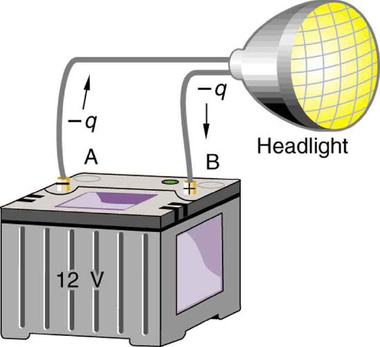
Voltage is not the same as energy. Voltage is the energy per unit charge. Thus a motorcycle battery and a car battery can both have the same voltage (more precisely, the same potential difference between battery terminals), yet one stores much more energy than the other since \(\Delta PE=q\Delta V\). The car battery can move more charge than the motorcycle battery, although both are 12 V batteries.

Example \(\PageIndex{1}\):Calculating Energy

Suppose you have a 12.0 V motorcycle battery that can move 5000 C of charge, and a 12.0 V car battery that can move 60,000 C of charge. How much energy does each deliver? (Assume that the numerical value of each charge is accurate to three significant figures.)

Strategy

To say we have a 12.0 V battery means that its terminals have a 12.0 V potential difference. When such a battery moves charge, it puts the charge through a potential difference of 12.0 V, and the charge is given a change in potential energy equal to \(\Delta PE=q\Delta V\).

So to find the energy output, we multiply the charge moved by the potential difference.

Solution

For the motorcycle battery, \(q=5000 \mathrm{C}\) and \(\Delta =12.0\mathrm{V}\). The total energy delivered by the motorcycle battery is

\[\Delta \mathrm{PE}_{cycle}=(5000\mathrm{C})(12.0\mathrm{V})\]

\[=(5000\mathrm{C})(12.0\mathrm{J/C})\]

\[=6.00\times 10^{4}\mathrm{J}.\]

Similarly, for the car battery, \(q=60,000\mathrm{C}\) and

\[\Delta \mathrm{PE}_{car}=(60,000\mathrm{C})(12.0\mathrm{V})\]

\[=7.20\times 10^{5}\mathrm{J}.\]

Discussion

While voltage and energy are related, they are not the same thing. The voltages of the batteries are identical, but the energy supplied by each is quite different. Note also that as a battery is discharged, some of its energy is used internally and its terminal voltage drops, such as when headlights dim because of a low car battery. The energy supplied by the battery is still calculated as in this example, but not all of the energy is available for external use.

Note that the energies calculated in the previous example are absolute values. The change in potential energy for the battery is negative, since it loses energy. These batteries, like many electrical systems, actually move negative charge—electrons in particular. The batteries repel electrons from their negative terminals (A) through whatever circuitry is involved and attract them to their positive terminals (B) as shown in Figure \(\PageIndex{2}\). The change in potential is \(\Delta V =V_{B}-V_{A}=+12\mathrm{V}\) and the charge \(q\) is negative, so that \(\Delta \mathrm{PE}=q\Delta V\) is negative, meaning the potential energy of the battery has decreased when \(q\) has moved from A to B.

Figure \(\PageIndex{2}\): A battery moves negative charge from its negative terminal through a headlight to its positive terminal. Appropriate combinations of chemicals in the battery separate charges so that the negative terminal has an excess of negative charge, which is repelled by it and attracted to the excess positive charge on the other terminal. In terms of potential, the positive terminal is at a higher voltage than the negative. Inside the battery, both positive and negative charges move.

Example \(\PageIndex{2}\): How Many Electrons Move through a Headlight Each Second?

When a 12.0 V car battery runs a single 30.0 W headlight, how many electrons pass through it each second?

Strategy

To find the number of electrons, we must first find the charge that moved in 1.00 s. The charge moved is related to voltage and energy through the equation \(\Delta \mathrm{PE}=q\Delta V\). A 30.0 W lamp uses 30.0 joules per second. Since the battery loses energy, we have \(\Delta \mathrm{PE}=-30.0J\) and, since the electrons are going from the negative terminal to the positive, we see that \(\Delta V=+12.0V\).

Solution

To find the charge \(q\) moved, we solve the equation \(\Delta \mathrm{PE}=q\Delta V\):

\[q=\dfrac{\Delta \mathrm{PE}}{\Delta V}.\]

Entering the values for \(\Delta PE\) and \(\Delta V\), we get

\[q=\dfrac{-30.0\mathrm{J}}{+12.0\mathrm{V}}=\dfrac{-30.0\mathrm{J}}{+12.0\mathrm{J/C}}=-2.50\mathrm{C}.\]

The number of electrons \(n_{e}\) is the total charge divided by the charge per electron. That is,

\[n_{e}=\dfrac{-2.50\mathrm{C}}{-1.60\times 10^{-19}\mathrm{C/e^{-}}}=1.56\times 10^{19} \mathrm{electrons}.\]

Discussion

This is a very large number. It is no wonder that we do not ordinarily observe individual electrons with so many being present in ordinary systems. In fact, electricity had been in use for many decades before it was determined that the moving charges in many circumstances were negative. Positive charge moving in the opposite direction of negative charge often produces identical effects; this makes it difficult to determine which is moving or whether both are moving.

The Electron Volt

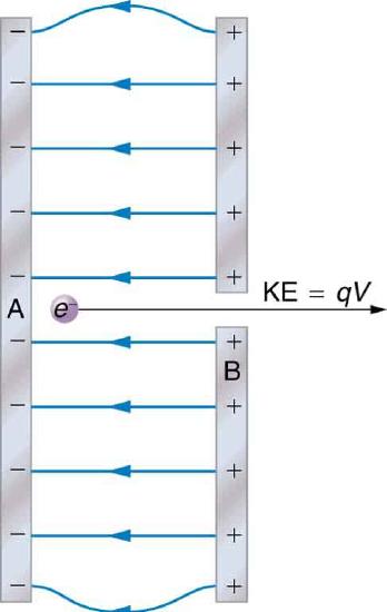
The energy per electron is very small in macroscopic situations like that in the previous example—a tiny fraction of a joule. But on a submicroscopic scale, such energy per particle (electron, proton, or ion) can be of great importance. For example, even a tiny fraction of a joule can be great enough for these particles to destroy organic molecules and harm living tissue. The particle may do its damage by direct collision, or it may create harmful x rays, which can also inflict damage. It is useful to have an energy unit related to submicroscopic effects. Figure \(\PageIndex{3}\) shows a situation related to the definition of such an energy unit. An electron is accelerated between two charged metal plates as it might be in an old-model television tube or oscilloscope. The electron is given kinetic energy that is later converted to another form—light in the television tube, for example. (Note that downhill for the electron is uphill for a positive charge.) Since energy is related to voltage by \(\Delta PE=q\Delta V\) we can think of the joule as a coulomb-volt.

Figure \(\PageIndex{3}\): A typical electron gun accelerates electrons using a potential difference between two metal plates. The energy of the electron in electron volts is numerically the same as the voltage between the plates. For example, a 5000 V potential difference produces 5000 eV electrons.

On the submicroscopic scale, it is more convenient to define an energy unit called the electron volt (eV), which is the energy given to a fundamental charge accelerated through a potential difference of 1 V. In equation form,

\[1\mathrm{ev}=(1.60\times 10^{-19}\mathrm{C})(1\mathrm{V})=(1.60\times 10^{-19}\mathrm{C})(1\mathrm{J/C})\]

\[=1.60\times 10^{-19}J.\]

ELECTRON VOLT

On the submicroscopic scale, it is more convenient to define an energy unit called the electron volt (eV), which is the energy given to a fundamental charge accelerated through a potential difference of 1 V. In equation form,

\[1 \mathrm{eV}=(1.60\times 10^{-19} \mathrm{C})(1 \mathrm{V})=(1.60\times 10^{-19} \mathrm{C}) (1\mathrm{J/C})\]

\[=1.60\times 10^{-19} \mathrm{C}\]

An electron accelerated through a potential difference of 1 V is given an energy of 1 eV. It follows that an electron accelerated through 50 V is given 50 eV. A potential difference of 100,000 V (100 kV) will give an electron an energy of 100,000 eV (100 keV), and so on. Similarly, an ion with a double positive charge accelerated through 100 V will be given 200 eV of energy. These simple relationships between accelerating voltage and particle charges make the electron volt a simple and convenient energy unit in such circumstances.

CONNECTIONS: ENERGY UNITS

The electron volt (eV) is the most common energy unit for submicroscopic processes. This will be particularly noticeable in the chapters on modern physics. Energy is so important to so many subjects that there is a tendency to define a special energy unit for each major topic. There are, for example, calories for food energy, kilowatt-hours for electrical energy, and therms for natural gas energy.

The electron volt is commonly employed in submicroscopic processes—chemical valence energies and molecular and nuclear binding energies are among the quantities often expressed in electron volts. For example, about 5 eV of energy is required to break up certain organic molecules. If a proton is accelerated from rest through a potential difference of 30 kV, it is given an energy of 30 keV (30,000 eV) and it can break up as many as 6000 of these molecules ( \(30,000 \mathrm{eV}\div 5\mathrm{eV}\) per molecule \(=6000\) molecules). Nuclear decay energies are on the order of 1 MeV (1,000,000 eV) per event and can, thus, produce significant biological damage.

Conservation of Energy

The total energy of a system is conserved if there is no net addition (or subtraction) of work or heat transfer. For conservative forces, such as the electrostatic force, conservation of energy states that mechanical energy is a constant.

Mechanical energy is the sum of the kinetic energy and potential energy of a system; that is, \(KE + PE=\: \mathrm{constant}\). A loss of PE of a charged particle becomes an increase in its KE. Here PE is the electric potential energy. Conservation of energy is stated in equation form as

\[\mathrm{KE}+\mathrm{PE}=\mathrm{constant}\]

or

\[\mathrm{KE}_{i}+\mathrm{PE}_{i}=\mathrm{KE}_{f}+\mathrm{PE}_{f},\]

where i and f stand for initial and final conditions. As we have found many times before, considering energy can give us insights and facilitate problem solving.

Example \(\PageIndex{3}\): Electrical Potential Energy Converted to Kinetic Energy

Calculate the final speed of a free electron accelerated from rest through a potential difference of 100 V. (Assume that this numerical value is accurate to three significant figures.)

Strategy

We have a system with only conservative forces. Assuming the electron is accelerated in a vacuum, and neglecting the gravitational force (we will check on this assumption later), all of the electrical potential energy is converted into kinetic energy. We can identify the initial and final forms of energy to be \(\mathrm{KE}_{i}=0,\mathrm{KE}_{f}=\dfrac{1}{2}mv^{2}, \mathrm{PE}_{i}=qV,\: \mathrm{and}\: \mathrm{PE}_{f}=0\).

Solution

Conservation of energy states that

\[\mathrm{KE}_{i}+\mathrm{PE}_{i}=\mathrm{KE}_{f}+\mathrm{PE}_{f}\]

Entering the forms identified above, we obtain

\[qV=\dfrac{mv^{2}}{2}.\]

We solve this for \(v\):

\[v=\sqrt {\dfrac{2qV}{m}}.\]

Entering values for \(q,\: V,\: \mathrm{and}\: m\) gives

\[v=\sqrt{\dfrac{2(-1.60\times 10^{-19}\mathrm{C})(-100 \mathrm{J/C})}{9.11\times 10^{-31}\mathrm{kg}}}\]

\[=5.93\times 10^{6} \mathrm{m/s}.\]

Discussion

Note that both the charge and the initial voltage are negative, as in Figure. From the discussions in Electric Charge and Electric Field, we know that electrostatic forces on small particles are generally very large compared with the gravitational force. The large final speed confirms that the gravitational force is indeed negligible here. The large speed also indicates how easy it is to accelerate electrons with small voltages because of their very small mass. Voltages much higher than the 100 V in this problem are typically used in electron guns. Those higher voltages produce electron speeds so great that relativistic effects must be taken into account. That is why a low voltage is considered (accurately) in this example.

Summary

• Electric potential is potential energy per unit charge.
• The potential difference between points A and B, \(V_{\mathrm{B}}-V_{\mathrm{A}}\), defined to be the change in potential energy of a charge \(q\) moved from A to B, is equal to the change in potential energy divided by the charge, Potential difference is commonly called voltage, represented by the symbol \(\Delta V\).

\(\Delta V= \dfrac{\Delta \mathrm{PE}}{q}\: \mathrm{and}\: \Delta \mathrm{PE}=q\Delta V.\)

• An electron volt is the energy given to a fundamental charge accelerated through a potential difference of 1 V. In equation form,

\(1\mathrm{eV}=(1.60\times 10^{-19}\mathrm{C})(1 \mathrm{V})=(1.60\times 10^{-19}\mathrm{C})(1 \mathrm{J/C})\)

\(=1.60\times 10^{-19}\mathrm{J}.\)

• Mechanical energy is the sum of the kinetic energy and potential energy of a system, that is, \(\mathrm{KE}+\mathrm{PE}\) This sum is a constant.

Glossary

electric potential

potential energy per unit charge

potential difference (or voltage)

change in potential energy of a charge moved from one point to another, divided by the charge; units of potential difference are joules per coulomb, known as volt

electron volt

the energy given to a fundamental charge accelerated through a potential difference of one volt

mechanical energy

sum of the kinetic energy and potential energy of a system; this sum is a constant