3.4: Electric Field

LEARNING OBJECTIVES

By the end of this section, you will be able to:

• Explain the purpose of the electric field concept
• Describe the properties of the electric field
• Calculate the field of a collection of source charges of either sign
• Explain the purpose of an electric field diagram
• Describe the relationship between a vector diagram and a field line diagram
• Explain the rules for creating a field diagram and why these rules make physical sense
• Sketch the field of an arbitrary source charge
• Describe a permanent dipole
• Describe an induced dipole
• Define and calculate an electric dipole moment
• Explain the physical meaning of the dipole moment

As we showed in the preceding section, the net electric force on a test charge is the vector sum of all the electric forces acting on it, from all of the various source charges, located at their various positions. But what if we use a different test charge, one with a different magnitude, or sign, or both? Or suppose we have a dozen different test charges we wish to try at the same location? We would have to calculate the sum of the forces from scratch. Fortunately, it is possible to define a quantity, called the electric field, which is independent of the test charge. It only depends on the configuration of the source charges, and once found, allows us to calculate the force on any test charge.

Defining a Field

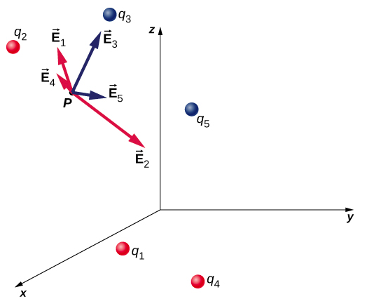
Suppose we have \(N\) source charges \(q_1, q_2, q_3, . . . q_N\) located at positions \(vec{r}_1, \vec{r}_2, \vec{r}_3, . . . \vec{r}_N\), applying \(N\) electrostatic forces on a test charge \(Q\). The net force on \(Q\) is

\[ \begin{align} \vec{F} &= \vec{F}_1 + \vec{F}_2 +\vec{F}_3 + . . . + \vec{F}_N \\[4pt] &= \dfrac{1}{4 \pi \epsilon_0}\left(\dfrac{Qq_1}{r_1^2}\hat{r}_1 + \dfrac{Qq_2}{r_2^2}\hat{r}_2 + \dfrac{Qq_3}{r_3^2}\hat{r}_3 + . . . + \dfrac{Qq_N}{r_1^2}\hat{r}_N\right) \\[4pt] &= Q\left[\dfrac{1}{4 \pi \epsilon_0}\left(\dfrac{q_1}{r_1^2}\hat{r}_1 + \dfrac{q_2}{r_2^2}\hat{r}_2 + \dfrac{q_3}{r_3^2}\hat{r}_3 + . . . + \dfrac{q_N}{r_1^2}\hat{r}_N\right)\right] \end{align}\]

We can rewrite this as

\[\vec{F} = Q \vec{E} \label{Efield1}\]

where

\[\vec{E} \equiv \dfrac{1}{4 \pi \epsilon_0}\left(\dfrac{q_1}{r_1^2}\hat{r}_1 + \dfrac{q_2}{r_2^2}\hat{r}_2 + \dfrac{q_3}{r_3^2}\hat{r}_3 + . . . + \dfrac{q_N}{r_1^2}\hat{r}_N\right) \label{Efield2}\]

or, more compactly,

\[\vec{E}(P) \equiv \dfrac{1}{4 \pi \epsilon_0} \sum_{i=1}^N \dfrac{q_i}{r_i^2}\hat{r}_i. \label{Efield3}\]

This expression is called the electric field at position \(P = P(x, y, z)\) of the \(N\) source charges. Here, \(P\) is the location of the point in space where you are calculating the field and is relative to the positions \(\vec{r}_i\) of the source charges (Figure \(\PageIndex{1}\)). Note that we have to impose a coordinate system to solve actual problems.

Figure \(\PageIndex{1}\): Each of these five source charges creates its own electric field at every point in space; shown here are the field vectors at an arbitrary point P. Like the electric force, the net electric field obeys the superposition principle.

Notice that the calculation of the electric field makes no reference to the test charge. Thus, the physically useful approach is to calculate the electric field and then use it to calculate the force on some test charge later, if needed. Different test charges experience different forces Equation \ref{Efield1}, but it is the same electric field Equation \ref{Efield3}. That being said, recall that there is no fundamental difference between a test charge and a source charge; these are merely convenient labels for the system of interest. Any charge produces an electric field; however, just as Earth’s orbit is not affected by Earth’s own gravity, a charge is not subject to a force due to the electric field it generates. Charges are only subject to forces from the electric fields of other charges.

In this respect, the electric field \(\vec{E}\) of a point charge is similar to the gravitational field \(\vec{g}\) of Earth; once we have calculated the gravitational field at some point in space, we can use it any time we want to calculate the resulting force on any mass we choose to place at that point. In fact, this is exactly what we do when we say the gravitational field of Earth (near Earth’s surface) has a value of \(8.81 \, m/s^2\) and then we calculate the resulting force (i.e., weight) on different masses. Also, the general expression for calculating \(\vec{g}\) at arbitrary distances from the center of Earth (i.e., not just near Earth’s surface) is very similar to the expression for \(E\):

\[\vec{g} = G\dfrac{M}{r^2}\hat{r}\]

where \(G\) is a proportionality constant, playing the same role for \(\vec{g}\) as \(\dfrac{1}{4\pi \epsilon_0}\) does for \(\vec{E}\). The value of \(\vec{g}\) is calculated once and is then used in an endless number of problems.

To push the analogy further, notice the units of the electric field: From \(F = QE\), the units of E are newtons per coulomb, N/C, that is, the electric field applies a force on each unit charge. Now notice the units of g: From \(\omega = mg\) the units of g are newtons per kilogram, N/kg, that is, the gravitational field applies a force on each unit mass. We could say that the gravitational field of Earth, near Earth’s surface, has a value of 9.81 N/kg.

The Meaning of “Field

Recall from your studies of gravity that the word “field” in this context has a precise meaning. A field, in physics, is a physical quantity whose value depends on (is a function of) position, relative to the source of the field. In the case of the electric field, Equation \ref{Efield3} shows that the value of \(\vec{E}\) (both the magnitude and the direction) depends on where in space the point \(P\) is located, measured from the locations \(\vec{r}_i\) of the source charges \(q_i\).

In addition, since the electric field is a vector quantity, the electric field is referred to as a vector field. (The gravitational field is also a vector field.) In contrast, a field that has only a magnitude at every point is a scalar field. The temperature in a room is an example of a scalar field. It is a field because the temperature, in general, is different at different locations in the room, and it is a scalar field because temperature is a scalar quantity.

Also, as you did with the gravitational field of an object with mass, you should picture the electric field of a charge-bearing object (the source charge) as a continuous, immaterial substance that surrounds the source charge, filling all of space—in principle, to \(\pm \infty\) in all directions. The field exists at every physical point in space. To put it another way, the electric charge on an object alters the space around the charged object in such a way that all other electrically charged objects in space experience an electric force as a result of being in that field. The electric field, then, is the mechanism by which the electric properties of the source charge are transmitted to and through the rest of the universe. (Again, the range of the electric force is infinite.)

We will see in subsequent chapters that the speed at which electrical phenomena travel is the same as the speed of light. There is a deep connection between the electric field and light.

Superposition

Yet another experimental fact about the field is that it obeys the superposition principle. In this context, that means that we can (in principle) calculate the total electric field of many source charges by calculating the electric field of only \(q_1\) at position P, then calculate the field of \(q_2\) at P, while—and this is the crucial idea—ignoring the field of, and indeed even the existence of, \(q_1\). We can repeat this process, calculating the field of each individual source charge, independently of the existence of any of the other charges. The total electric field, then, is the vector sum of all these fields. That, in essence, is what Equation \ref{Efield3} says.

In the next section, we describe how to determine the shape of an electric field of a source charge distribution and how to sketch it.

The Direction of the Field

Equation \ref{Efield3} enables us to determine the magnitude of the electric field, but we need the direction also. We use the convention that the direction of any electric field vector is the same as the direction of the electric force vector that the field would apply to a positive test charge placed in that field. Such a charge would be repelled by positive source charges (the force on it would point away from the positive source charge) but attracted to negative charges (the force points toward the negative source).

Direction of the Electric Field

By convention, all electric fields \(\vec{E}\) point away from positive source charges and point toward negative source charges.

Electric Field Lines

Now that we have some experience calculating electric fields, let’s try to gain some insight into the geometry of electric fields. As mentioned earlier, our model is that the charge on an object (the source charge) alters space in the region around it in such a way that when another charged object (the test charge) is placed in that region of space, that test charge experiences an electric force. The concept of electric field lines, and of electric field line diagrams, enables us to visualize the way in which the space is altered, allowing us to visualize the field. The purpose of this section is to enable you to create sketches of this geometry, so we will list the specific steps and rules involved in creating an accurate and useful sketch of an electric field.

It is important to remember that electric fields are three-dimensional. Although in this book we include some pseudo-three-dimensional images, several of the diagrams that you’ll see (both here, and in subsequent chapters) will be two-dimensional projections, or cross-sections. Always keep in mind that in fact, you’re looking at a three-dimensional phenomenon.

Our starting point is the physical fact that the electric field of the source charge causes a test charge in that field to experience a force. By definition, electric field vectors point in the same direction as the electric force that a (hypothetical) positive test charge would experience, if placed in the field (Figure \(\PageIndex{5}\)).

Figure \(\PageIndex{5}\): The electric field of a positive point charge. A large number of field vectors are shown. Like all vector arrows, the length of each vector is proportional to the magnitude of the field at each point. (a) Field in two dimensions; (b) field in three dimensions.

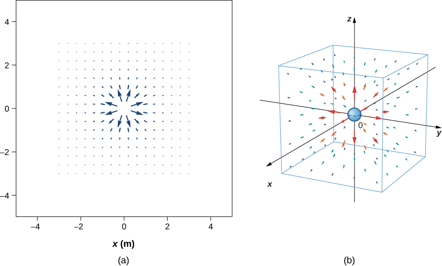
We’ve plotted many field vectors in the figure, which are distributed uniformly around the source charge. Since the electric field is a vector, the arrows that we draw correspond at every point in space to both the magnitude and the direction of the field at that point. As always, the length of the arrow that we draw corresponds to the magnitude of the field vector at that point. For a point source charge, the length decreases by the square of the distance from the source charge. In addition, the direction of the field vector is radially away from the source charge, because the direction of the electric field is defined by the direction of the force that a positive test charge would experience in that field. (Again, keep in mind that the actual field is three-dimensional; there are also field lines pointing out of and into the page.)

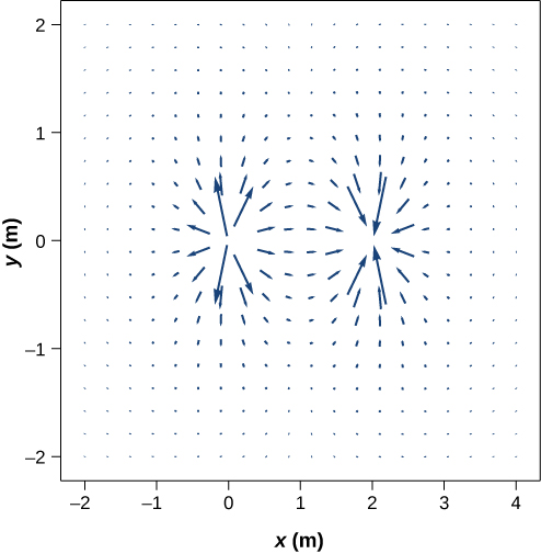
This diagram is correct, but it becomes less useful as the source charge distribution becomes more complicated. For example, consider the vector field diagram of a dipole (Figure \(\PageIndex{6}\)).

Figure \(\PageIndex{6}\): The vector field of a dipole. Even with just two identical charges, the vector field diagram becomes difficult to understand.

There is a more useful way to present the same information. Rather than drawing a large number of increasingly smaller vector arrows, we instead connect all of them together, forming continuous lines and curves, as shown in Figure \(\PageIndex{7}\).

Figure \(\PageIndex{7}\): (a) The electric field line diagram of a positive point charge. (b) The field line diagram of a dipole. In both diagrams, the magnitude of the field is indicated by the field line density. The field vectors (not shown here) are everywhere tangent to the field lines.

Although it may not be obvious at first glance, these field diagrams convey the same information about the electric field as do the vector diagrams. First, the direction of the field at every point is simply the direction of the field vector at that same point. In other words, at any point in space, the field vector at each point is tangent to the field line at that same point. The arrowhead placed on a field line indicates its direction.

As for the magnitude of the field, that is indicated by the field line density—that is, the number of field lines per unit area passing through a small cross-sectional area perpendicular to the electric field. This field line density is drawn to be proportional to the magnitude of the field at that cross-section. As a result, if the field lines are close together (that is, the field line density is greater), this indicates that the magnitude of the field is large at that point. If the field lines are far apart at the cross-section, this indicates the magnitude of the field is small. Figure \(\PageIndex{8}\) shows the idea.

Figure \(\PageIndex{8}\): Electric field lines passing through imaginary areas. Since the number of lines passing through each area is the same, but the areas themselves are different, the field line density is different. This indicates different magnitudes of the electric field at these points.

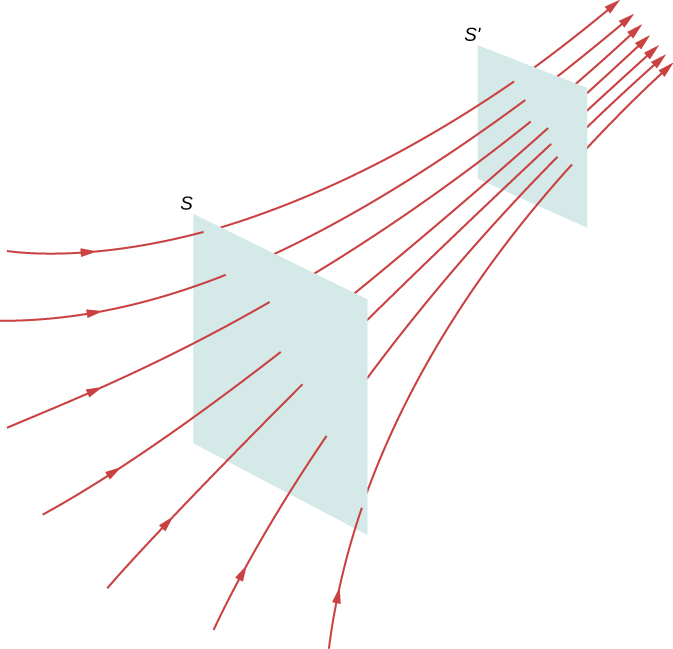
In Figure \(\PageIndex{8}\), the same number of field lines passes through both surfaces (S and \(S'\)), but the surface S is larger than surface \(S'\). Therefore, the density of field lines (number of lines per unit area) is larger at the location of \(S'\), indicating that the electric field is stronger at the location of \(S'\) than at S. The rules for creating an electric field diagram are as follows.

Problem-Solving Strategy: Drawing Electric Field Lines

1. Electric field lines either originate on positive charges or come in from infinity, and either terminate on negative charges or extend out to infinity.
2. The number of field lines originating or terminating at a charge is proportional to the magnitude of that charge. A charge of 2q will have twice as many lines as a charge of q.
3. At every point in space, the field vector at that point is tangent to the field line at that same point.
4. The field line density at any point in space is proportional to (and therefore is representative of) the magnitude of the field at that point in space.
5. Field lines can never cross. Since a field line represents the direction of the field at a given point, if two field lines crossed at some point, that would imply that the electric field was pointing in two different directions at a single point. This in turn would suggest that the (net) force on a test charge placed at that point would point in two different directions. Since this is obviously impossible, it follows that field lines must never cross.

Always keep in mind that field lines serve only as a convenient way to visualize the electric field; they are not physical entities. Although the direction and relative intensity of the electric field can be deduced from a set of field lines, the lines can also be misleading. For example, the field lines drawn to represent the electric field in a region must, by necessity, be discrete. However, the actual electric field in that region exists at every point in space.

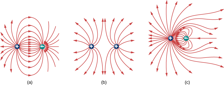
Field lines for three groups of discrete charges are shown in Figure \(\PageIndex{9}\). Since the charges in parts (a) and (b) have the same magnitude, the same number of field lines are shown starting from or terminating on each charge. In (c), however, we draw three times as many field lines leaving the \(+3q\) charge as entering the \(-q\). The field lines that do not terminate at \(-q\) emanate outward from the charge configuration, to infinity.

Figure \(\PageIndex{9}\): Three typical electric field diagrams. (a) A dipole. (b) Two identical charges. (c) Two charges with opposite signs and different magnitudes. Can you tell from the diagram which charge has the larger magnitude?

The ability to construct an accurate electric field diagram is an important, useful skill; it makes it much easier to estimate, predict, and therefore calculate the electric field of a source charge. The best way to develop this skill is with software that allows you to place source charges and then will draw the net field upon request. We strongly urge you to search the Internet for a program. Once you’ve found one you like, run several simulations to get the essential ideas of field diagram construction. Then practice drawing field diagrams, and checking your predictions with the computer-drawn diagrams.

Rotation of a Dipole due to an Electric Field

In example \(\PageIndex{1B}\) we discussed, and calculated, the electric field of a dipole: two equal and opposite charges that are “close” to each other. (In this context, “close” means that the distance d between the two charges is much, much less than the distance of the field point P, the location where you are calculating the field.) Let’s now consider what happens to a dipole when it is placed in an external field \(\vec{E}\). We assume that the dipole is a permanent dipole; it exists without the field, and does not break apart in the external field.

For now, we deal with only the simplest case: The external field is uniform in space. Suppose we have the situation depicted in Figure \(\PageIndex{1}\), where we denote the distance between the charges as the vector \(\vec{d}\), pointing from the negative charge to the positive charge.

Figure \(\PageIndex{1}\): A dipole in an external electric field. (a) The net force on the dipole is zero, but the net torque is not. As a result, the dipole rotates, becoming aligned with the external field. (b) The dipole moment is a convenient way to characterize this effect. The \(\vec{d}\) points in the same direction as \(\vec{p}\).

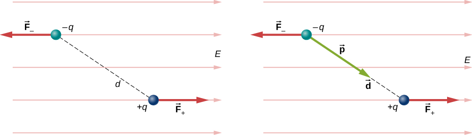
The forces on the two charges are equal and opposite, so there is no net force on the dipole. However, there is a torque:

\[\begin{align} \vec{r} &= \left(\dfrac{\vec{d}}{2} \times \vec{F}_+ \right) + \left(- \dfrac{\vec{d}}{2} \times \vec{F}_- \right) \\[4pt] &= \left[ \left(\dfrac{\vec{d}}{2}\right) \times \left(+q\vec{E}\right) + \left(-\dfrac{\vec{d}}{2}\right) \times \left(-q\vec{E}\right)\right] \\[4pt] &= q\vec{d} \times \vec{E}. \end{align}\]

The quantity \(qd\) (the magnitude of each charge multiplied by the vector distance between them) is a property of the dipole; its value, as you can see, determines the torque that the dipole experiences in the external field. It is useful, therefore, to define this product as the so-called dipole moment of the dipole:

\[\vec{p} \equiv q\vec{d}.\]

We can therefore write

\[\vec{r} = \vec{p} \times \vec{E}.\]

Recall that a torque changes the angular velocity of an object, the dipole, in this case. In this situation, the effect is to rotate the dipole (that is, align the direction of \(\vec{p}\)) so that it is parallel to the direction of the external field.

Induced Dipoles

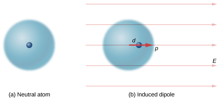
Neutral atoms are, by definition, electrically neutral; they have equal amounts of positive and negative charge. Furthermore, since they are spherically symmetrical, they do not have a “built-in” dipole moment the way most asymmetrical molecules do. They obtain one, however, when placed in an external electric field, because the external field causes oppositely directed forces on the positive nucleus of the atom versus the negative electrons that surround the nucleus. The result is a new charge distribution of the atom, and therefore, an induced dipole moment (Figure \(\PageIndex{2}\)).

Figure \(\PageIndex{2}\): A dipole is induced in a neutral atom by an external electric field. The induced dipole moment is aligned with the external field.

An important fact here is that, just as for a rotated polar molecule, the result is that the dipole moment ends up aligned parallel to the external electric field. Generally, the magnitude of an induced dipole is much smaller than that of an inherent dipole. For both kinds of dipoles, notice that once the alignment of the dipole (rotated or induced) is complete, the net effect is to decrease the total electric field

\[\vec{E}_{total} = \vec{E}_{external} + \vec{E}_{dipole}\]

in the regions outside the dipole charges (Figure \(\PageIndex{3}\)). By “outside” we mean further from the charges than they are from each other. This effect is crucial for capacitors, as you will see in Capacitance.

Figure \(\PageIndex{3}\): The net electric field is the vector sum of the field of the dipole plus the external field.

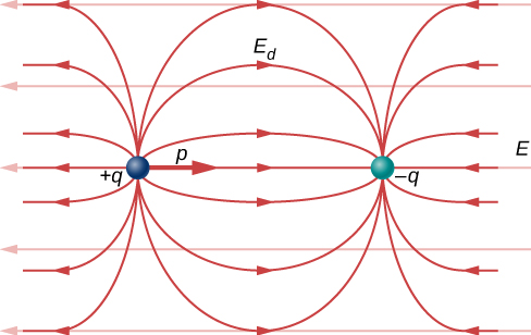
Recall that we found the electric field of a dipole in example \(\PageIndex{1B}\). If we rewrite it in terms of the dipole moment we get:

\[\vec{E}(z) = \dfrac{1}{4 \pi \epsilon_0} \dfrac{\vec{p}}{z^3}.\]

The form of this field is shown in Figure \(\PageIndex{3}\). Notice that along the plane perpendicular to the axis of the dipole and midway between the charges, the direction of the electric field is opposite that of the dipole and gets weaker the further from the axis one goes. Similarly, on the axis of the dipole (but outside it), the field points in the same direction as the dipole, again getting weaker the further one gets from the charges.

 

Examples

Example \(\PageIndex{1A}\): The E-field of an Atom

In an ionized helium atom, the most probable distance between the nucleus and the electron is \(r = 26.5 \times 10^{-12} m\). What is the electric field due to the nucleus at the location of the electron?

Strategy

Note that although the electron is mentioned, it is not used in any calculation. The problem asks for an electric field, not a force; hence, there is only one charge involved, and the problem specifically asks for the field due to the nucleus. Thus, the electron is a red herring; only its distance matters. Also, since the distance between the two protons in the nucleus is much, much smaller than the distance of the electron from the nucleus, we can treat the two protons as a single charge +2e (Figure \(\PageIndex{2}\)).

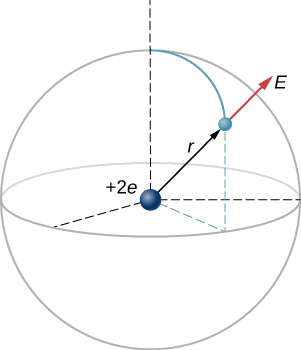
Figure \(\PageIndex{2}\): A schematic representation of a helium atom. Again, helium physically looks nothing like this, but this sort of diagram is helpful for calculating the electric field of the nucleus.

Solution

The electric field is calculated by

\[\vec{E} = \dfrac{1}{4 \pi \epsilon_0} \sum_{i=1}^N \dfrac{q_i}{r_i^2} \hat{r}_i. \nonumber\]

Since there is only one source charge (the nucleus), this expression simplifies to

\[\vec{E} = \dfrac{1}{4\pi \epsilon_0}\dfrac{q}{r^2}\hat{r}. \nonumber\]

Here, \(q = 2e = 2(1.6 \times 10^{-19} \, C)\) (since there are two protons) and r is given; substituting gives

\[ \begin{align*} \vec{E} &= \dfrac{1}{4\pi \left(8.85 \times 10^{-12} \dfrac{C^2}{N\cdot m^2}\right)} \dfrac{2(1.6 \times 10^{-19} C)}{26.5 \times 10^{-12}m)^2}\hat{r} \\[4pt] &= 4.1 \times 10^{12} \dfrac{N}{C}\hat{r}. \end{align*}\]

The direction of \(\vec{E}\) is radially away from the nucleus in all directions. Why? Because a positive test charge placed in this field would accelerate radially away from the nucleus (since it is also positively charged), and again, the convention is that the direction of the electric field vector is defined in terms of the direction of the force it would apply to positive test charges.

 

Example \(\PageIndex{1B}\): The E-Field above Two Equal Charges (Dipole)

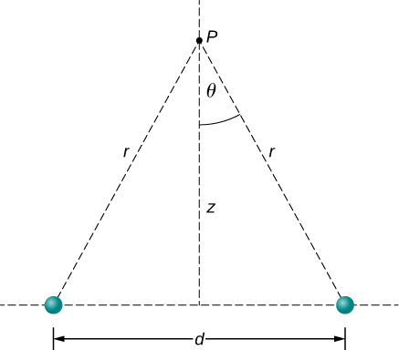
1. Find the electric field (magnitude and direction) a distance z above the midpoint between two equal charges \(+q\) that are a distance d apart (Figure \(\PageIndex{3}\)). Check that your result is consistent with what you’d expect when \(z \gg d\).
2. The same as part (a), only this time make the right-hand charge \(-q\) instead of \(+q\).

Figure \(\PageIndex{3}\): Finding the field of two identical source charges at the point \(P\). Due to the symmetry, the net field at \(P\) is entirely vertical. (Notice that this is not true away from the midline between the charges.)

Strategy

We add the two fields as vectors, per Equation \ref{Efield3}. Notice that the system (and therefore the field) is symmetrical about the vertical axis; as a result, the horizontal components of the field vectors cancel. This simplifies the math. Also, we take care to express our final answer in terms of only quantities that are given in the original statement of the problem: \(q\), \(z\), \(d\), and constants \((\pi, \epsilon_0)\).

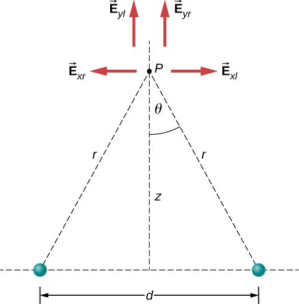
Figure \(\PageIndex{4}\). Note that the horizontal components of the electric fields from the two charges cancel each other out, while the vertical components add together.

Solution

a. By symmetry, the horizontal (x)-components of \(\vec{E}\) cancel (Figure \(\PageIndex{4}\));

\[ \begin{align*} E_x &= \dfrac{1}{4\pi \epsilon_0} \dfrac{q}{r^2} \, \sin \, \theta - \dfrac{1}{4\pi \epsilon_0} \dfrac{q}{r^2} \, \sin \, \theta \\[4pt] &= 0. \end{align*}\]

The vertical (z)-component is given by

\[ \begin{align*} E_z &= \dfrac{1}{4\pi \epsilon_0} \dfrac{q}{r^2} \, \cos \, \theta + \dfrac{1}{4\pi \epsilon_0} \dfrac{q}{r^2} \, \cos \, \theta \\[4pt] &= \dfrac{1}{4\pi \epsilon_0} \dfrac{2q}{r^2} \, \cos \, \theta. \end{align*}\]

Since none of the other components survive, this is the entire electric field, and it points in the \(\hat{k}\) direction. Notice that this calculation uses the principle of superposition; we calculate the fields of the two charges independently and then add them together.

What we want to do now is replace the quantities in this expression that we don’t know (such as \(r\)), or can’t easily measure (such as \(cos \, \theta\) with quantities that we do know, or can measure. In this case, by geometry,

\[r^2 = z^2 + \left(\dfrac{d}{2}\right)^2 \nonumber\]

and

\[\cos \, \theta = \dfrac{z}{R} = \dfrac{z}{\left[z^2 + \left(\dfrac{d}{2} \right)^2\right]^{1/2}}. \nonumber\]

Thus, substituting,

\[\vec{E}(z) = \dfrac{1}{4\pi \epsilon_0}\dfrac{2q}{\left[z^2 + \left(\dfrac{d}{2}\right)^2\right]^2} \dfrac{z}{\left[z^2 + \left(\dfrac{d}{2} \right)^2 \right]^{1/2}}\hat{k}. \nonumber\]

Simplifying, the desired answer is

\[\vec{E}(z) = \dfrac{1}{4\pi \epsilon_0}\dfrac{2qz}{\left[z^2 + \left(\dfrac{d}{2}\right)^2\right]^{3/2}} \hat{k}. \label{5.5}\]

b. If the source charges are equal and opposite, the vertical components cancel because

\[E_z = \dfrac{1}{4\pi \epsilon_0} \dfrac{q}{r^2} \, cos \, \theta - \dfrac{1}{4\pi \epsilon_0} \dfrac{q}{r^2} \, \cos \, \theta = 0 \nonumber\]

and we get, for the horizontal component of \(\vec{E}\).

\[\vec{E}(z) = \dfrac{1}{4\pi \epsilon_0} \dfrac{qd}{\left[z^2 + \left(\dfrac{d}{2}\right)^2\right]^{3/2}} \hat{i}.\label{5.6}\]

Significance

It is a very common and very useful technique in physics to check whether your answer is reasonable by evaluating it at extreme cases. In this example, we should evaluate the field expressions for the cases \(d = 0, \, z \gg d\), and \(z \rightarrow \infty\), and confirm that the resulting expressions match our physical expectations. Let’s do so:

Let’s start with Equation \ref{5.5}, the field of two identical charges. From far away (i.e., \(z >> d\)), the two source charges should “merge” and we should then “see” the field of just one charge, of size 2q. So, let \(z \gg d\); then we can neglect \(d^2\) in Equation \ref{5.5} to obtain

\[ \begin{align*} \lim_{d\rightarrow 0}\vec{E} &= \dfrac{1}{4\pi \epsilon_0} \dfrac{2qz}{[z^2]^{3/2}}\hat{k} \\[4pt] &= \dfrac{1}{4\pi \epsilon_0} \dfrac{2qz}{z^3}\hat{k} \\[4pt] &= \dfrac{1}{4\pi \epsilon_0} \dfrac{2q}{z^2}\hat{k}, \end{align*}\]

which is the correct expression for a field at a distance z away from a charge \(2q\).

Next, we consider the field of equal and opposite charges, Equation \ref{5.6}. It can be shown (via a Taylor expansion) that for \(d \ll z \ll \infty\), , this becomes

\[\vec{E}(z) = \dfrac{1}{4\pi \epsilon_0} \dfrac{qd}{z^3}\hat{i}, \nonumber\]

which is the field of a dipole, a system that we will study in more detail later in this section. (Note that the units of \(\vec{E}\) are still correct in this expression, since the units of d in the numerator cancel the unit of the “extra” z in the denominator.) If z is very large \((z \rightarrow \infty)\), then \(E \rightarrow 0\), as it should; the two charges “merge” and so cancel out.

Exercise \(\PageIndex{1}\)

What is the electric field due to a single point particle?

Answer

\[\vec{E} = \dfrac{1}{4 \pi \epsilon_0} \dfrac{q}{r^2} \hat{r} \nonumber\]