
3.2: Electric Potential and Potential Difference


- Last updated
- Jan 22, 2024
- Save as PDF

( \newcommand{\kernel}{\mathrm{null}\,}\)
By the end of this section, you will be able to:
- Define electric potential, voltage, and potential difference
- Define the electron-volt
- Calculate electric potential and potential difference from potential energy and electric field
- Describe systems in which the electron-volt is a useful unit
- Apply conservation of energy to electric systems
Recall that earlier we defined electric field to be a quantity independent of the test charge in a given system, which would nonetheless allow us to calculate the force that would result on an arbitrary test charge. (The default assumption in the absence of other information is that the test charge is positive.) We briefly defined a field for gravity, but gravity is always attractive, whereas the electric force can be either attractive or repulsive. Therefore, although potential energy is perfectly adequate in a gravitational system, it is convenient to define a quantity that allows us to calculate the work on a charge independent of the magnitude of the charge. Calculating the work directly may be difficult, since W=→F⋅→d and the direction and magnitude of →F can be complex for multiple charges, for odd-shaped objects, and along arbitrary paths. But we do know that because →F, the work, and hence ΔU is proportional to the test charge q. To have a physical quantity that is independent of test charge, we define electric potential V (or simply potential, since electric is understood) to be the potential energy per unit charge:
The electric potential energy per unit charge is
V=Uq.
Since U is proportional to q, the dependence on q cancels. Thus, V does not depend on q. The change in potential energy ΔU is crucial, so we are concerned with the difference in potential or potential difference ΔV between two points, where
The electric potential difference between points A and B, VB−VA is defined to be the change in potential energy of a charge q moved from A to B, divided by the charge. Units of potential difference are joules per coulomb, given the name volt (V) after Alessandro Volta.
1V=1J/C
The familiar term voltage is the common name for electric potential difference. Keep in mind that whenever a voltage is quoted, it is understood to be the potential difference between two points. For example, every battery has two terminals, and its voltage is the potential difference between them. More fundamentally, the point you choose to be zero volts is arbitrary. This is analogous to the fact that gravitational potential energy has an arbitrary zero, such as sea level or perhaps a lecture hall floor. It is worthwhile to emphasize the distinction between potential difference and electrical potential energy.
The relationship between potential difference (or voltage) and electrical potential energy is given by
ΔV=ΔUq
or
ΔU=qΔV.
Voltage is not the same as energy. Voltage is the energy per unit charge. Thus, a motorcycle battery and a car battery can both have the same voltage (more precisely, the same potential difference between battery terminals), yet one stores much more energy than the other because ΔU=qΔV. The car battery can move more charge than the motorcycle battery, although both are 12-V batteries.
You have a 12.0-V motorcycle battery that can move 5000 C of charge, and a 12.0-V car battery that can move 60,000 C of charge. How much energy does each deliver? (Assume that the numerical value of each charge is accurate to three significant figures.)
- Strategy
-
To say we have a 12.0-V battery means that its terminals have a 12.0-V potential difference. When such a battery moves charge, it puts the charge through a potential difference of 12.0 V, and the charge is given a change in potential energy equal to ΔU=qΔV. To find the energy output, we multiply the charge moved by the potential difference.
- Solution
-
For the motorcycle battery, q=5000C and ΔV=12.0V. The total energy delivered by the motorcycle battery is
ΔUcycle=(5000C)(12.0V)=(5000C)(12.0J/C)=6.00×104J.
Similarly, for the car battery, q=60,000C and
ΔUcar=(60,000C)(12.0V)=7.20×10⁵J.
Significance
Voltage and energy are related, but they are not the same thing. The voltages of the batteries are identical, but the energy supplied by each is quite different. A car battery has a much larger engine to start than a motorcycle. Note also that as a battery is discharged, some of its energy is used internally and its terminal voltage drops, such as when headlights dim because of a depleted car battery. The energy supplied by the battery is still calculated as in this example, but not all of the energy is available for external use.
How much energy does a 1.5-V AAA battery have that can move 100 C?
- Answer
-
ΔU=qΔV=(100C)(1.5V)=150J
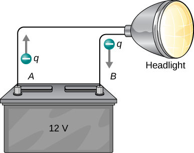
Note that the energies calculated in the previous example are absolute values. The change in potential energy for the battery is negative, since it loses energy. These batteries, like many electrical systems, actually move negative charge—electrons in particular. The batteries repel electrons from their negative terminals (A) through whatever circuitry is involved and attract them to their positive terminals (B), as shown in Figure 3.2.1. The change in potential is ΔV=VB−VA=+12V and the charge q is negative, so that ΔU=qΔV is negative, meaning the potential energy of the battery has decreased when q has moved from A to B.
When a 12.0-V car battery powers a single 30.0-W headlight, how many electrons pass through it each second?
- Strategy
-
To find the number of electrons, we must first find the charge that moves in 1.00 s. The charge moved is related to voltage and energy through the equations ΔU=qΔV. A 30.0-W lamp uses 30.0 joules per second. Since the battery loses energy, we have ΔU=−30J and, since the electrons are going from the negative terminal to the positive, we see that ΔV=+12.0V.
- Solution
-
To find the charge q moved, we solve the equation ΔU=qΔV:
q=ΔUΔV.
Entering the values for ΔU and ΔV, we get
q=−30.0J+12.0V=−30.0J+12.0J/C=−2.50C.
The number of electrons ne is the total charge divided by the charge per electron. That is,
ne=−2.50C−1.60×10⁻¹⁹C/e−=1.56×1019electrons.
Significance
This is a very large number. It is no wonder that we do not ordinarily observe individual electrons with so many being present in ordinary systems. In fact, electricity had been in use for many decades before it was determined that the moving charges in many circumstances were negative. Positive charge moving in the opposite direction of negative charge often produces identical effects; this makes it difficult to determine which is moving or whether both are moving.
How many electrons would go through a 24.0-W lamp?
- Answer
-
−2.00C,ne=1.25×10¹⁹electrons
The Electron-Volt
The energy per electron is very small in macroscopic situations like that in the previous example—a tiny fraction of a joule. But on a submicroscopic scale, such energy per particle (electron, proton, or ion) can be of great importance. For example, even a tiny fraction of a joule can be great enough for these particles to destroy organic molecules and harm living tissue. The particle may do its damage by direct collision, or it may create harmful X-rays, which can also inflict damage. It is useful to have an energy unit related to submicroscopic effects.
Figure 3.2.2 shows a situation related to the definition of such an energy unit. An electron is accelerated between two charged metal plates, as it might be in an old-model television tube or oscilloscope. The electron gains kinetic energy that is later converted into another form—light in the television tube, for example. (Note that in terms of energy, “downhill” for the electron is “uphill” for a positive charge.) Since energy is related to voltage by ΔU=qΔV, we can think of the joule as a coulomb-volt.
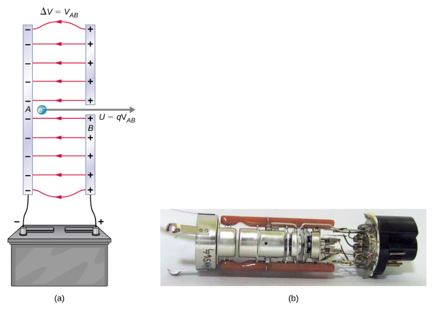
On the submicroscopic scale, it is more convenient to define an energy unit called the electron-volt (eV), which is the energy given to a fundamental charge accelerated through a potential difference of 1 V. In equation form,
1eV=(1.60×10⁻¹⁹C)(1V)=(1.60×10⁻¹⁹C)(1J/C)=1.60×10−19J.
An electron accelerated through a potential difference of 1 V is given an energy of 1 eV. It follows that an electron accelerated through 50 V gains 50 eV. A potential difference of 100,000 V (100 kV) gives an electron an energy of 100,000 eV (100 keV), and so on. Similarly, an ion with a double positive charge accelerated through 100 V gains 200 eV of energy. These simple relationships between accelerating voltage and particle charges make the electron-volt a simple and convenient energy unit in such circumstances.
The electron-volt is commonly employed in submicroscopic processes—chemical valence energies and molecular and nuclear binding energies are among the quantities often expressed in electron-volts. For example, about 5 eV of energy is required to break up certain organic molecules. If a proton is accelerated from rest through a potential difference of 30 kV, it acquires an energy of 30 keV (30,000 eV) and can break up as many as 6000 of these molecules (30,000eV:5eVpermolecule=6000molecules). Nuclear decay energies are on the order of 1 MeV (1,000,000 eV) per event and can thus produce significant biological damage.
Conservation of Energy
The total energy of a system is conserved if there is no net addition (or subtraction) due to work or heat transfer. For conservative forces, such as the electrostatic force, conservation of energy states that mechanical energy is a constant.
Mechanical energy is the sum of the kinetic energy and potential energy of a system; that is, K+U=constant. A loss of U for a charged particle becomes an increase in its K. Conservation of energy is stated in equation form as
K+U=constant or Ki+Ui=Kf+Uf
where i and f stand for initial and final conditions. As we have found many times before, considering energy can give us insights and facilitate problem solving.
a) Calculate the final speed of a free electron accelerated from rest through a potential difference of 100 V. (Assume that this numerical value is accurate to three significant figures.)
b) How would this example change with a positron? A positron is identical to an electron except the charge is positive.
- Strategy
-
We have a system with only conservative forces. Assuming the electron is accelerated in a vacuum, and neglecting the gravitational force (we will check on this assumption later), all of the electrical potential energy is converted into kinetic energy. We can identify the initial and final forms of energy to be
Ki=0, Kf=12mv2, Ui=qV, Uf=0.
- Solution
-
a) Conservation of energy states that
Ki+Ui=Kf+Uf.
Entering the forms identified above, we obtain
qV=mv22.
We solve this for v:
v=√2qVm.
Entering values for q, V, and m gives
v=√2(−1.60×10⁻¹⁹C)(−100J/C)9.11×10−31kg=5.93×106m/s.
b) It would be going in the opposite direction, with no effect on the calculations as presented.
Significance
Note that both the charge and the initial voltage are negative, as in Figure 3.2.2. From the discussion of electric charge and electric field, we know that electrostatic forces on small particles are generally very large compared with the gravitational force. The large final speed confirms that the gravitational force is indeed negligible here. The large speed also indicates how easy it is to accelerate electrons with small voltages because of their very small mass. Voltages much higher than the 100 V in this problem are typically used in electron guns. These higher voltages produce electron speeds so great that effects from special relativity must be taken into account and will be discussed elsewhere. That is why we consider a low voltage (accurately) in this example.
Voltage and Electric Field
So far, we have explored the relationship between voltage and energy. Now we want to explore the relationship between voltage and electric field. We will start with the general case for a non-uniform →E field. Recall that our general formula for the potential energy of a test charge q at point P relative to reference point R is
Up=−∫pR→F⋅d→l.
When we substitute in the definition of electric field (→E=→F/q), this becomes
Up=−q∫pR→E⋅d→l.
Applying our definition of potential (V=U/q) to this potential energy, we find that, in general,
Vp=−∫pR→E⋅d→l.
Vp=−∫pR→E⋅d→l.
From our previous discussion of the potential energy of a charge in an electric field, the result is independent of the path chosen, and hence we can pick the integral path that is most convenient.
Consider the special case of a positive point charge q at the origin. To calculate the potential caused by q at a distance r from the origin relative to a reference of 0 at infinity (recall that we did the same for potential energy), let P=r and R=∞, with d→l=d→r=ˆrdr and use →E=kqr2ˆr. When we evaluate the integral
Vp=−∫pR→E⋅d→l for this system, we have
Vr=−∫r∞kqr2dr=kqr−kq∞=kqr.
This result,
Vr=kqr
is the standard form of the potential of a point charge. This will be explored further in the next section.
To examine another interesting special case, suppose a uniform electric field →E is produced by placing a potential difference (or voltage) ΔV across two parallel metal plates, labeled A and B (Figure 3.2.3). Examining this situation will tell us what voltage is needed to produce a certain electric field strength. It will also reveal a more fundamental relationship between electric potential and electric field.
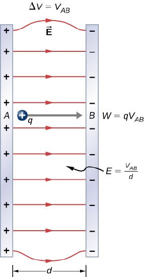
From a physicist’s point of view, either ΔV or →E can be used to describe any interaction between charges. However, ΔV is a scalar quantity and has no direction, whereas →E is a vector quantity, having both magnitude and direction. (Note that the magnitude of the electric field, a scalar quantity, is represented by E.) The relationship between ΔV and →E is revealed by calculating the work done by the electric force in moving a charge from point A to point B. But, as noted earlier, arbitrary charge distributions require calculus. We therefore look at a uniform electric field as an interesting special case.
The work done by the electric field in Figure 3.2.3 to move a positive charge q from A, the positive plate, higher potential, to B, the negative plate, lower potential, is
W=−ΔU=−qΔV.
The potential difference between points A and B is
−ΔV=−(VB−VA)=VA−VB=VAB.
Entering this into the expression for work yields
W=qVAB.
Work is W=→F⋅→d=Fdcosθ: here cosθ=1, since the path is parallel to the field. Thus, W=Fd. Since F=qE we see that W=qEd.
Substituting this expression for work into the previous equation gives
qEd=qVAB.
The charge cancels, so we obtain for the voltage between points A and B.
VAB=Ed E=VABd where d is the distance from A to B, or the distance between the plates in Figure 3.2.3.
Note that this equation implies that the units for electric field are volts per meter. We already know the units for electric field are newtons per coulomb; thus, the following relation among units is valid:
1N/C=1V/m.
Furthermore, we may extend this to the integral form. Substituting Equation ??? into our definition for the potential difference between points A and B, we obtain
VAB=VB−VA=−∫BR→E⋅d→l+∫AR→E⋅d→l
which simplifies to
VB−VA=−∫BA→E⋅d→l.
As a demonstration, from this we may calculate the potential difference between two points (A and B) equidistant from a point charge q at the origin, as shown in Figure 3.2.4.
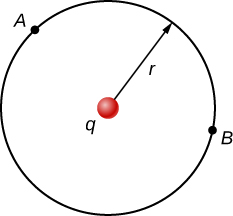
To do this, we integrate around an arc of the circle of constant radius r between A and B, which means we let d→l=rˆφdφ, while using →E=kqr2ˆr. Thus,
ΔV=VB−VA=−∫BA→E⋅d→l.
for this system becomes
VB−VA=−∫BAkqr2⋅rˆφdφ.
However, ˆr⋅ˆφ and therefore
VB−VA=0.
This result, that there is no difference in potential along a constant radius from a point charge, will come in handy when we map potentials.
Dry air can support a maximum electric field strength of about 3.0×10⁶V/m. Above that value, the field creates enough ionization in the air to make the air a conductor. This allows a discharge or spark that reduces the field. What, then, is the maximum voltage between two parallel conducting plates separated by 2.5 cm of dry air?
- Strategy
-
We are given the maximum electric field E between the plates and the distance d between them. We can use the equation VAB=Ed to calculate the maximum voltage.
- Solution
-
The potential difference or voltage between the plates is
VAB=Ed.
Entering the given values for E and d gives
VAB=(3.0×10⁶V/m)(0.025m)=7.5×104V or VAB=75kV.
(The answer is quoted to only two digits, since the maximum field strength is approximate.)
Significance
One of the implications of this result is that it takes about 75 kV to make a spark jump across a 2.5-cm (1-in.) gap, or 150 kV for a 5-cm spark. This limits the voltages that can exist between conductors, perhaps on a power transmission line. A smaller voltage can cause a spark if there are spines on the surface, since sharp points have larger field strengths than smooth surfaces. Humid air breaks down at a lower field strength, meaning that a smaller voltage will make a spark jump through humid air. The largest voltages can be built up with static electricity on dry days (Figure 3.2.5).
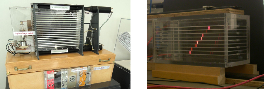
Figure 3.2.5: A spark chamber is used to trace the paths of high-energy particles. Ionization created by the particles as they pass through the gas between the plates allows a spark to jump. The sparks are perpendicular to the plates, following electric field lines between them. The potential difference between adjacent plates is not high enough to cause sparks without the ionization produced by particles from accelerator experiments (or cosmic rays). This form of detector is now archaic and no longer in use except for demonstration purposes. (credit b: modification of work by Jack Collins)
An electron gun (Figure 3.2.2) has parallel plates separated by 4.00 cm and gives electrons 25.0 keV of energy. (a) What is the electric field strength between the plates? (b) What force would this field exert on a piece of plastic with a 0.500−μC charge that gets between the plates?
- Strategy
-
- Strategy
-
Since the voltage and plate separation are given, the electric field strength can be calculated directly from the expression E=VABd. Once we know the electric field strength, we can find the force on a charge by using →F=q→E. Since the electric field is in only one direction, we can write this equation in terms of the magnitudes, F=qE.
Solution
a. The expression for the magnitude of the electric field between two uniform metal plates is
E=VABd. Since the electron is a single charge and is given 25.0 keV of energy, the potential difference must be 25.0 kV. Entering this value for VAB and the plate separation of 0.0400 m, we obtain E=25.0kV0.0400m=6.25×10⁵V/m.
b. The magnitude of the force on a charge in an electric field is obtained from the equation F=qE. Substituting known values gives
F=(0.500×10⁻⁶C)(6.25×10⁵V/m)=0.313N.
Significance Note that the units are newtons, since 1V/m=1N/C. Because the electric field is uniform between the plates, the force on the charge is the same no matter where the charge is located between the plates.
Given a point charge q=+2.0−nC at the origin, calculate the potential difference between point P1 a distance a=4.0cm from q, and P2 a distance b=12.0cm from q, where the two points have an angle of φ=24o between them (Figure 3.2.6).
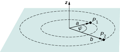
- Strategy
-
Do this in two steps. The first step is to use VB−VA=−∫BA→E⋅d→l and let A=a=4.0cm (point P1) and B=b=12.0cm (point P0, not marked, in the direction of ˆa but a distance b away) , with d→l=d→r=ˆrdr and →E=kqr2ˆr. Then perform the integral.
The second step is to integrate VB−VA=−∫BA→E⋅d→l around an arc of constant radius r, which means we let d→l=r→φdφ with limits 0≤φ≤24o, still using →E=kqr2ˆr.Then add the two results together.
- Solution
-
For the first part, VB−VA=−∫BA→E⋅d→l for this system becomes Vb−Va=−∫bakqr2ˆr⋅ˆrdr which computes to
ΔV=−∫bakqr2dr=kq[1b−1a]
=(8.99×10⁹Nm2/C2)(2.0×10−9C)[10.12m−10.040m]=−300V.
For the second step, VB−VA=−∫BA→E⋅d→l becomes ΔV=−∫24o0okqr2ˆr⋅rˆφdφ, but ˆr⋅ˆφ=0 and therefore ΔV=0. Adding the two parts together, we get 300 V.
Significance/Important
We have demonstrated the use of the integral form of the potential difference to obtain a numerical result. Notice that, in this particular system, we could have also used the formula for the potential due to a point charge at the two points and simply taken the difference.
ΔV=VP2−VP1=kqb−kqa=(8.99×10⁹Nm2/C2)(2.0×10−9C)[10.12m−10.040m]=−300V
- Examine the situation to determine if static electricity is involved; this may concern separated stationary charges, the forces among them, and the electric fields they create.
- Identify the system of interest. This includes noting the number, locations, and types of charges involved.
- Identify exactly what needs to be determined in the problem (identify the unknowns). A written list is useful. Determine whether the Coulomb force is to be considered directly—if so, it may be useful to draw a free-body diagram, using electric field lines.
- Make a list of what is given or can be inferred from the problem as stated (identify the knowns). It is important to distinguish the Coulomb force F from the electric field E, for example.
- Solve the appropriate equation for the quantity to be determined (the unknown) or draw the field lines as requested.
- Examine the answer to see if it is reasonable: Does it make sense? Are units correct and the numbers involved reasonable?
Calculations of Electric Potential
The electric potential due to a point charge is can be deduced from ???.
The electric potential V of a point charge is given by
V=kqr⏟point charge
The potential in Equation ??? at infinity is chosen to be zero. Thus, V for a point charge decreases with distance, whereas →E for a point charge decreases with distance squared:
E=Fqt=kqr2
Recall that the electric potential V is a scalar and has no direction, whereas the electric field →E is a vector. To find the voltage due to a combination of point charges, you add the individual voltages as numbers. To find the total electric field, you must add the individual fields as vectors, taking magnitude and direction into account. This is consistent with the fact that V is closely associated with energy, a scalar, whereas →E is closely associated with force, a vector.
Charges in static electricity are typically in the nanocoulomb (nC) to microcoulomb (μC) range. What is the voltage 5.00 cm away from the center of a 1-cm-diameter solid metal sphere that has a –3.00-nC static charge?
- Strategy
-
As we discussed in Electric Charges and Fields, charge on a metal sphere spreads out uniformly and produces a field like that of a point charge located at its center. Thus, we can find the voltage using the equation V=kqr.
- Solution
-
Entering known values into the expression for the potential of a point charge (Equation ???), we obtain
V=kqr=(9.00×10⁹N⋅m2/C2)(−3.00×10−9C5.00×10−2m)=−539V.
Significance
The negative value for voltage means a positive charge would be attracted from a larger distance, since the potential is lower (more negative) than at larger distances. Conversely, a negative charge would be repelled, as expected.
A demonstration Van de Graaff generator has a 25.0-cm-diameter metal sphere that produces a voltage of 100 kV near its surface (Figure).
a) What excess charge resides on the sphere? (Assume that each numerical value here is shown with three significant figures.)
b) What is the potential inside the metal sphere?
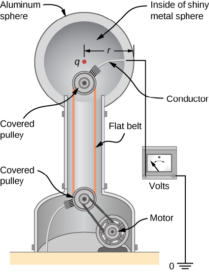
- Strategy
-
The potential on the surface is the same as that of a point charge at the center of the sphere, 12.5 cm away. (The radius of the sphere is 12.5 cm.) We can thus determine the excess charge using Equation ???
V=kqr.
- Solution
-
a) Solving for q and entering known values gives
q=rVk=(0.125m)(100×103V)8.99×10⁹N⋅m2/C2=1.39×10−6C=1.39μC.
b) V=kqr=(8.99×10⁹N⋅m2/C2)(−3.00×10−9C5.00×10−3m)=−5390V
Recall that the electric field inside a conductor is zero. Hence, any path from a point on the surface to any point in the interior will have an integrand of zero when calculating the change in potential, and thus the potential in the interior of the sphere is identical to that on the surface.
Significance
This is a relatively small charge, but it produces a rather large voltage. We have another indication here that it is difficult to store isolated charges.
The voltages in both of these examples could be measured with a meter that compares the measured potential with ground potential. Ground potential is often taken to be zero (instead of taking the potential at infinity to be zero). It is the potential difference between two points that is of importance, and very often there is a tacit assumption that some reference point, such as Earth or a very distant point, is at zero potential. As noted earlier, this is analogous to taking sea level as h=0 when considering gravitational potential energy Ug=mgh.
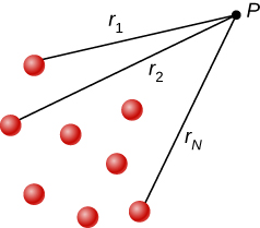
Systems of Multiple Point Charges
Just as the electric field obeys a superposition principle, so does the electric potential. Consider a system consisting of N charges q1,q2,...,qN. What is the net electric potential V at a space point P from these charges? Each of these charges is a source charge that produces its own electric potential at point P, independent of whatever other changes may be doing. Let V1,V2,...,VN be the electric potentials at P produced by the charges q1,q2,...,qN, respectively. Then, the net electric potential Vp at that point is equal to the sum of these individual electric potentials. You can easily show this by calculating the potential energy of a test charge when you bring the test charge from the reference point at infinity to point P:
Vp=V1+V2+...+VN=N∑1Vi.
Note that electric potential follows the same principle of superposition as electric field and electric potential energy. To show this more explicitly, note that a test charge qi at the point P in space has distances of r1,r2,...,rN from the N charges fixed in space above, as shown in Figure 3.2.2. Using our formula for the potential of a point charge for each of these (assumed to be point) charges, we find that
Vp=N∑1kqiri=kN∑1qiri.
Therefore, the electric potential energy of the test charge is
Up=qtVp=qtkN∑1qiri, which is the same as the work to bring the test charge into the system, as found in the first section of the chapter.
An electric dipole is a system of two equal but opposite charges a fixed distance apart. This system is used to model many real-world systems, including atomic and molecular interactions. One of these systems is the water molecule, under certain circumstances. These circumstances are met inside a microwave oven, where electric fields with alternating directions make the water molecules change orientation. This vibration is the same as heat at the molecular level.
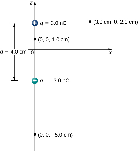
Consider the dipole in Figure 3.2.3 with the charge magnitude of q=3.0μC and separation distance d=4.0cm.
a) What is the potential at the following locations in space? (a) (0, 0, 1.0 cm); (b) (0, 0, –5.0 cm); (c) (3.0 cm, 0, 2.0 cm).
d) What is the potential on the x-axis?
- Strategy
-
Apply Vp=k∑N1qiri to each of these three points.
- Solution
-
a. Vp=k∑N1qiri=(9.0×10⁹N⋅m2/C2)(3.0 nC0.010m−3.0 nC0.030m)=1.8×10³V
b. Vp=k∑N1qiri=(9.0×10⁹N⋅m2/C2)(3.0 nC0.070m−3.0 nC0.030m)=−5.1×10²V
c. Vp=k∑N1qiri=(9.0×10⁹N⋅m2/C2)(3.0 nC0.030m−3.0 nC0.050m)=3.6×10²V
d. The x-axis the potential is zero, due to the equal and opposite charges the same distance from it.
Significance
Note that evaluating potential is significantly simpler than electric field, due to potential being a scalar instead of a vector.
Potential of Continuous Charge Distributions
We have been working with point charges a great deal, but what about continuous charge distributions? Recall from Equation ??? that
Vp=k∑qiri.
We may treat a continuous charge distribution as a collection of infinitesimally separated individual points. This yields the integral
Vp=∫dqr
Vp=∫dqr
for the potential at a point P. Note that r is the distance from each individual point in the charge distribution to the point P. As we saw in Electric Charges and Fields, the infinitesimal charges are given by
dq=λdl⏟onedimension
dq=σdA⏟twodimensions
dq=ρdV ⏟threedimensions
where λ is linear charge density, σ is the charge per unit area, and ρ is the charge per unit volume.
Find the electric potential of a uniformly charged, nonconducting wire with linear density λ (coulomb/meter) and length L at a point that lies on a line that divides the wire into two equal parts.
- Strategy
-
To set up the problem, we choose Cartesian coordinates in such a way as to exploit the symmetry in the problem as much as possible. We place the origin at the center of the wire and orient the y-axis along the wire so that the ends of the wire are at y=±L/2. The field point P is in the xy-plane and since the choice of axes is up to us, we choose the x-axis to pass through the field point P, as shown in Figure 3.2.6.
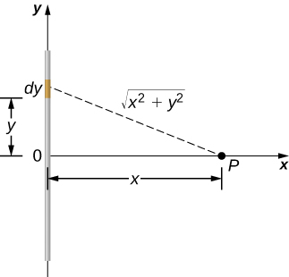
Figure 3.2.6: We want to calculate the electric potential due to a line of charge. - Solution
-
Consider a small element of the charge distribution between y and y+dy. The charge in this cell is dq=λdy and the distance from the cell to the field point P is √x2+y2. Therefore, the potential becomes
Vp=k∫dqr=k∫L/2−L/2λdy√x2+y2=kλ[ln(y+√y2+x2)]L/2−L/2=kλ[ln((L2)+√(L2)2+x2)−ln((−L2)+√(−L2)2+x2)]=kλln[L+√L2+4x2−L+√L2+4x2].
Significance
Note that this was simpler than the equivalent problem for electric field, due to the use of scalar quantities. Recall that we expect the zero level of the potential to be at infinity, when we have a finite charge. To examine this, we take the limit of the above potential as x approaches infinity; in this case, the terms inside the natural log approach one, and hence the potential approaches zero in this limit. Note that we could have done this problem equivalently in cylindrical coordinates; the only effect would be to substitute r for x and z for y.
A ring has a uniform charge density λ, with units of coulomb per unit meter of arc. Find the electric potential at a point on the axis passing through the center of the ring.
- Strategy
-
We use the same procedure as for the charged wire. The difference here is that the charge is distributed on a circle. We divide the circle into infinitesimal elements shaped as arcs on the circle and use cylindrical coordinates shown in Figure 3.2.7.
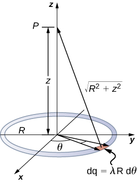
Figure 3.2.7: We want to calculate the electric potential due to a ring of charge. - Solution
-
A general element of the arc between θ and θ+dθ is of length Rdθ and therefore contains a charge equal to λRdθ. The element is at a distance of √z2+R2 from P, and therefore the potential is
Vp=k∫dqr=k∫2π0λRdθ√z2+R2=kλR√z2+R2∫2π0dθ=2πkλR√z2+R2=kqtot√z2+R2.
Significance
This result is expected because every element of the ring is at the same distance from point P. The net potential at P is that of the total charge placed at the common distance, √z2+R2.
A disk of radius R has a uniform charge density σ with units of coulomb meter squared. Find the electric potential at any point on the axis passing through the center of the disk.
- Strategy
-
We divide the disk into ring-shaped cells, and make use of the result for a ring worked out in the previous example, then integrate over r in addition to θ. This is shown in Figure 3.2.8.
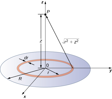
Figure 3.2.8: We want to calculate the electric potential due to a disk of charge. - Solution
-
An infinitesimal width cell between cylindrical coordinates r and r+dr shown in Figure 3.2.8 will be a ring of charges whose electric potential dVp at the field point has the following expression
dVp=kdq√z2+r2
where
dq=σ2πrdr.
The superposition of potential of all the infinitesimal rings that make up the disk gives the net potential at point P. This is accomplished by integrating from r=0 to r=R:
Vp=∫dVp=k2πσ∫R0rdr√z2+r2,=k2πσ(√z2+R2−√z2).
Significance
The basic procedure for a disk is to first integrate around ? and then over r. This has been demonstrated for uniform (constant) charge density. Often, the charge density will vary with r, and then the last integral will give different results.
Find the electric potential due to an infinitely long uniformly charged wire.
- Strategy
-
Since we have already worked out the potential of a finite wire of length L in Example 3.2.4, we might wonder if taking L→∞ in our previous result will work:
Vp=lim
However, this limit does not exist because the argument of the logarithm becomes [2/0] as L \rightarrow \infty, so this way of finding V of an infinite wire does not work. The reason for this problem may be traced to the fact that the charges are not localized in some space but continue to infinity in the direction of the wire. Hence, our (unspoken) assumption that zero potential must be an infinite distance from the wire is no longer valid.
To avoid this difficulty in calculating limits, let us use the definition of potential by integrating over the electric field from the previous section, and the value of the electric field from this charge configuration from the previous chapter.
- Solution
-
We use the integral
V_p = - \int_R^p \vec{E} \cdot d\vec{l}
where R is a finite distance from the line of charge, as shown in Figure \PageIndex{9}.
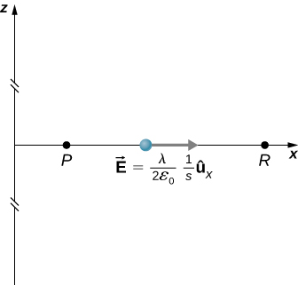
Figure \PageIndex{9}: Points of interest for calculating the potential of an infinite line of charge. With this setup, we use \vec{E}_p = 2k \lambda \dfrac{1}{s} \hat{s} and d\vec{l} = d\vec{s} to obtain
\begin{align} V_p - V_R &= - \int_R^p 2k\lambda \dfrac{1}{s}ds \nonumber \\[4pt] &= -2 k \lambda \ln\dfrac{s_p}{s_R}. \nonumber \end{align} \nonumber
Now, if we define the reference potential V_R = 0 at s_R = 1 \, m, this simplifies to
V_p = -2 k\lambda \, \ln \, s_p.
Note that this form of the potential is quite usable; it is 0 at 1 m and is undefined at infinity, which is why we could not use the latter as a reference.
Significance
Although calculating potential directly can be quite convenient, we just found a system for which this strategy does not work well. In such cases, going back to the definition of potential in terms of the electric field may offer a way forward.
What is the potential on the axis of a nonuniform ring of charge, where the charge density is \lambda (\theta) = \lambda \, \cos \, \theta?
- Solution
-
It will be zero, as at all points on the axis, there are equal and opposite charges equidistant from the point of interest. Note that this distribution will, in fact, have a dipole moment.