
1.3: Measurements, Uncertainty and Significant Figures


- Last updated
- Aug 27, 2023
- Save as PDF
( \newcommand{\kernel}{\mathrm{null}\,}\)
- Determine the correct number of significant figures for the result of a computation.
- Describe the relationship between the concepts of accuracy, precision, uncertainty, and discrepancy.
- Calculate the percent uncertainty of a measurement, given its value and its uncertainty.
- Determine the uncertainty of the result of a computation involving quantities with given uncertainties.
Science is based on data. That is evidence obtained from observation and experiments. Thus, it is important to have a clear, universal, thorough process and rules that we use when collecting data —that is, when making measurements and when reporting those results.
Accuracy and Precision of a Measurement
Accuracy is how close a measurement is to the accepted reference value for that measurement. For example, let’s say we want to measure the length of standard printer paper. The packaging in which we purchased the paper states that it is 11.0 in. long. We then measure the length of the paper three times and obtain the following measurements: 11.1 in., 11.2 in., and 10.9 in. These measurements are quite accurate because they are very close to the reference value of 11.0 in. In contrast, if we had obtained a measurement of 12 in., our measurement would not be very accurate. Notice that the concept of accuracy requires that an accepted reference value be given.
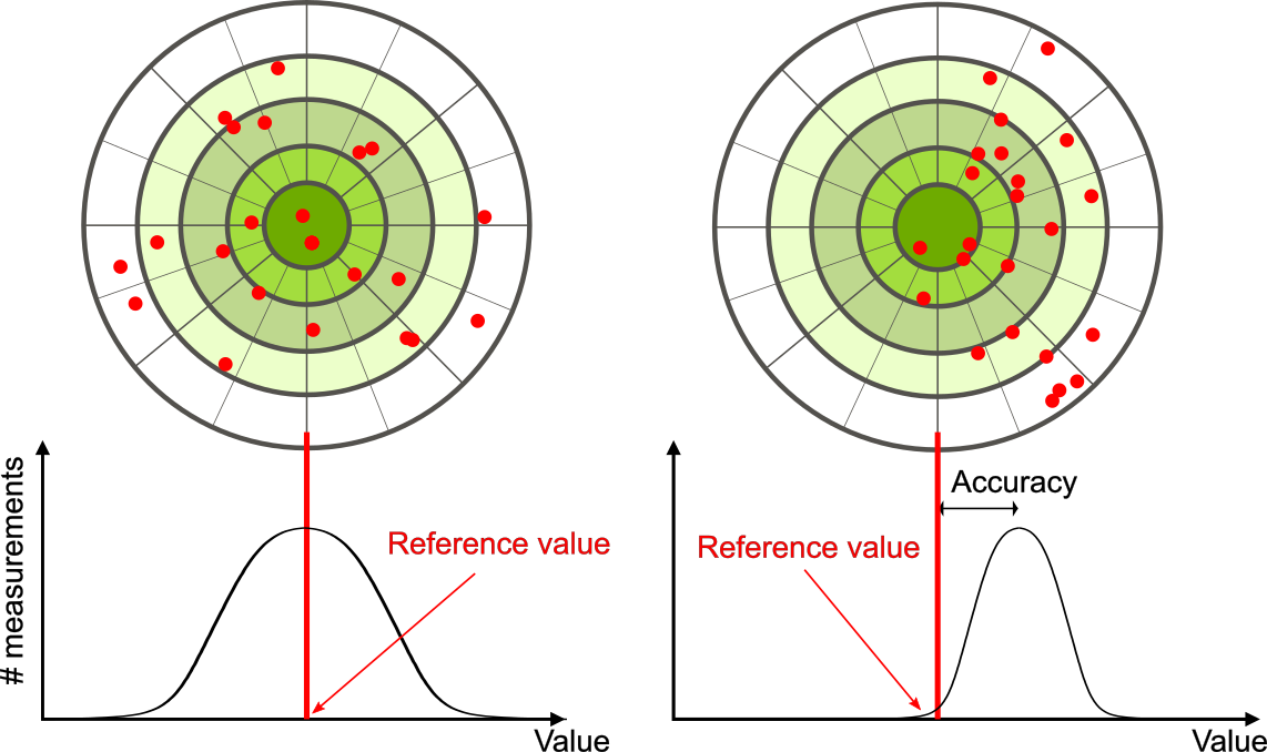
Let’s consider an example of a GPS attempting to locate the position of a restaurant in a city. Think of the restaurant location as existing at the center of a bull’s-eye target and think of each GPS attempt to locate the restaurant as a red dot. On the left of Figure 1.3.1, we see the GPS measurements are spread out far apart from each other, but they are all relatively close to the actual location of the restaurant at the center of the target. This indicates a high-accuracy measurement. However, in the image on the right, the GPS measurements are concentrated closer to one another, but they are far away from the target location. This indicates a low-accuracy measuring system.
The precision of measurements refers to how close the agreement is between repeated independent measurements (which are repeated under the same conditions). Consider the example of the paper measurements. The precision of the measurements refers to the spread of the measured values. One way to analyze the precision of the measurements is to determine the range, or difference, between the lowest and the highest measured values. In this case, the lowest value was 10.9 in. and the highest value was 11.2 in. Thus, the measured values deviated from each other by, at most, 0.3 in. These measurements were relatively precise because they did not vary too much in value. However, if the measured values had been 10.9 in., 11.1 in., and 11.9 in., then the measurements would not be very precise because there would be significant variation from one measurement to another. Notice that the concept of precision depends only on the actual measurements acquired and does not depend on an accepted reference value.
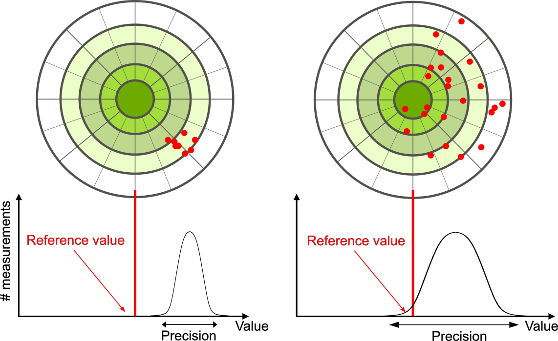
The measurements in the paper example are both accurate and precise, but in some cases, measurements are accurate but not precise, or they are precise but not accurate. Referring back to the GPS example, on the left of Figure 1.3.2 in this case, we see the GPS measurements clustered close to each other, while far away from the target location. This indicates a high-precision measurement even though the accuracy is low. For the image on the right, the GPS measurements are spread further apart from one another, they are still far away from the target location. This indicates a low-precision and also a low-accuracy measurement.
The precision of a measuring system is related to the uncertainty in the measurements whereas the accuracy is related to the discrepancy from the accepted reference value. uncertainty is a quantitative measure of how much your measured values deviate from one another. Discrepancy is the difference between the measured value and a given standard or expected value. If the measurements are not very precise, then the uncertainty of the values is high. If the measurements are not very accurate, then the discrepancy of the values is high.
Recall our example of measuring paper length; we obtained measurements of 11.1 in., 11.2 in., and 10.9 in., and the accepted value was 11.0 in. We might average the three measurements to say our best guess is 11.1 in.; in this case, our discrepancy is 11.1 – 11.0 = 0.1 in., which provides a quantitative measure of accuracy. We might calculate the uncertainty in our best guess by using the range of our measured values: 0.3 in. Then we would say the length of the paper is 11.1 in. plus or minus 0.3 in. The uncertainty in a measurement, A, is often denoted as δA (read “delta A”), so the measurement result would be recorded as A ± δA. Returning to our paper example, the measured length of the paper could be expressed as 11.1 ± 0.3 in. Since the discrepancy of 0.1 in. is less than the uncertainty of 0.3 in., we might say the measured value agrees with the accepted reference value to within experimental uncertainty.
Some factors that contribute to uncertainty in a measurement include the following:
- Limitations of the measuring device
- The skill of the person taking the measurement
- Irregularities in the object being measured
- Any other factors that affect the outcome (highly dependent on the situation)
In our example, such factors contributing to the uncertainty could be the smallest division on the ruler is 1/16 in., the person using the ruler has bad eyesight, the ruler is worn down on one end, or one side of the paper is slightly longer than the other. At any rate, the uncertainty in a measurement must be calculated to quantify its precision. If a reference value is known, it makes sense to calculate the discrepancy as well to quantify its accuracy.
Significant Figures
When we express measured values, we can only list as many digits as we measured initially with our measuring tool. For example, if we use a standard ruler to measure the length of a stick, we may measure it to be 36.7 cm. We can’t express this value as 36.71 cm because our measuring tool is not precise enough to measure a hundredth of a centimeter. It should be noted that the last digit in a measured value has been estimated in some way by the person performing the measurement. For example, the person measuring the length of a stick with a ruler notices the stick length seems to be somewhere in between 36.6 cm and 36.7 cm, and he or she must estimate the value of the last digit. Using the method of significant figures, the rule is that the last digit written down in a measurement is the first digit with some uncertainty. To determine the number of significant digits in a value, start with the first measured value at the left and count the number of digits through the last digit written on the right. For example, the measured value 36.7 cm has three digits, or three significant figures.
Rules for Determining the number of significant figures
Here are some general rules for determining the number of significant figures:
- For experimental data the uncertainty in a quantity defines how many figures are significant.
- In general, the uncertainty in a measurement is equal to the estimated standard deviation for that measurement.
- The reading uncertainty is an estimate made by the experimenter
- In the case where the reading uncertainty in a measurement is larger than the estimated standard deviation, the reading uncertainty is the uncertainty in each individual measurement.
- The reading uncertainty almost by definition has one and only one significant figure.
- Thus uncertainties are specified to one or at most two digits.
Express the following quantities to the correct number of significant figures:
(a) 29.625 ± 2.345
(b) 74 ± 7.136
(c) 84.26351 ± 3
- Strategy
-
First, remember that the uncertainty should be specified to one or at the most two digits.
Second, express the quantity with the same precision as the uncertainty.
- Solution
-
Rounding the uncertainty to one digit:
(a) 29.625 ± 2
(b) 74 ± 7
(c) 84.26351 ± 3Rounding the quantity to the same precision as the uncertainty:
(a) 30 ± 2
(b) 74 ± 7
(c) 84 ± 3
Rules for Zeroes
Special consideration is given to zeros when counting significant figures. The zeros in 0.053 are not significant because they are placeholders that locate the decimal point. There are two significant figures in 0.053. The zeros in 10.053 are not placeholders; they are significant. This number has five significant figures. The zeros in 1300 may or may not be significant, depending on the style of writing numbers. They could mean the number is known to the last digit or they could be placeholders. So 1300 could have two, three, or four significant figures. To avoid this ambiguity, we should write 1300 in scientific notation as 1.3 x 10³, 1.30 x 10³, or 1.300 x 10³, depending on whether it has two, three, or four significant figures. Zeros are significant except when they serve only as placeholders
When combining measurements with different degrees of precision, the number of significant digits in the final answer can be no greater than the number of significant digits in the least-precise measured value. Here are the rules:
Rules for Manipulating Numbers
Rule 1: When multiplying or dividing, report the result with the same number of significant figures as the least certain value. For example:
11.5 x 2.1 = 24
11.5 ÷ 2.1 = 5.5
because 2.1 has only two significant figures.
Rule 2: When adding or subtracting, the number of decimal places in the result should equal the smallest number of decimal places in any of the given terms. For example:
12.34+2.006-8.9=5.4
because 8.9 has only one decimal place.
Rule 3: Numbers that are not measured may be considered exact. Irrational numbers such as π and e are known to many significant figures and do not limit your results. For example:
(1/3)(4.56 π) = 4.78
is reported to three significant figures because neither 3 nor π is measured, and our answer is limited only by the three significant figures of 4.56.
Rule 4: It is best to use scientific notation because a zero that acts as a placeholder is not necessarily a significant figure. For example, h = 120 m may have two or three significant figures. To avoid that ambiguity, you may add a decimal point; for example, h = 120. m has three significant figures. A better way to clarify the number of significant figures is to use scientific notation: h = 1.20 x 10² m has three significant figures, and h = 1.2 x 10² m has two significant figures.
Rule 5: You should keep extra significant figures in intermediate steps when making a calculation, but you should round the final answer to the correct number of significant figures. The extra significant figures in an intermediate result help avoid introducing an error due to rounding a number up or down. This step is particularly important if an intermediate result is a number ending in 5
Precision of Measuring Tools and Significant Figures
As mentioned in the previous sections, an important factor in the precision of measurements involves the precision of the measuring tool. In general, a precise measuring tool is one that can measure values in very small increments. For example, a standard ruler can measure length to the nearest millimeter whereas a caliper can measure length to the nearest 0.01 mm. The caliper is a more precise measuring tool because it can measure extremely small differences in length. The more precise the measuring tool, the more precise the measurements.
The result of a single measurement should be reported in the format (estimate)±(measurement uncertainty). The estimate is your best guess for the true value, while the measurement uncertainty states the range where the true value might lie. By convention, the estimate and measurement uncertainty follow these rules :
- The measurement uncertainty has one or two significant figures. We will use just one for the rest of this chapter.
- The estimate has the same precision as the measurement uncertainty.
Suppose you use a digital multimeter to measure the current in a circuit, and the readout is stable (i.e., not fluctuating). Then you should report a result like this:
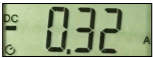 =(0.320±0.005)A
Why? According to the readout, the value is between 0.315A (rounded up to 0.32A) and 0.324999…A (which is rounded down). So the measurement uncertainty is ±0.005A. Note that the estimate is reported as 0.320A to have the same precision as the uncertainty.
When using a device with hatch marks, such as a ruler or analog oscilloscope display, the measurement uncertainty is determined by the smallest markings. For example, if the smallest markings on a ruler have 1mm spacing, the measurement uncertainty is ±0.5mm, so a reading should be reported like this:
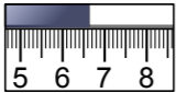 =(6.60±0.05)cm
In more complicated situations, you must exercise your judgment. For instance, suppose you have a digital multimeter reading that is not stable: the last digit changes constantly, so that the reading fluctuates between 0.32, 0.33, and 0.34A. The value is between 0.315A and 0.344999…A, which is a range of ±0.015A. Since we use one significant figure for uncertainty, the result is reported like this:
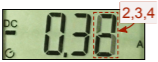 =(0.33±0.02)A
Alternatively, suppose the last digit is changing so fast that you can’t make out its values at all. Then you can report the result like this:
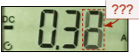 =(0.35±0.05)A
Measurement uncertainties can also come from other aspects of an experiment. Suppose you use a ruler to measure the distance to an object, but the object wobbles by ±2mm, larger than the 1mm hatch marks of the ruler. In that case, you should report a measurement uncertainty of ±2mm, not ±0.05mm.
Uncertainties in Calculations/Propagation of uncertainty of Precision
Often we have two or more measured quantities that we combine arithmetically to get some result. Examples include dividing a distance by a time to get a speed, or adding two lengths to get a total length. Now that we have learned how to determine the uncertainty in the directly measured quantities we need to learn how these uncertainty propagate to an uncertainty in the result.
We assume that the two directly measured quantities are x and Y, with uncertainty Δx and Δy respectively.
The measurements x and y must be independent of each other.
The fractional uncertainty is the value of the uncertainty divided by the value of the quantity: Δxx. The fractional uncertainty multiplied by 100 is the percentage uncertainty. Everything is this section assumes that the uncertainty is "small" compared to the value itself, i.e. that the fractional uncertainty is much less than one.
For many situations, we can find the uncertainty in the result z using three simple rules:
Rule 1
If: z=x+y or z=x−y
then:
Δz=√Δx2+Δy2
In words, this says that the uncertainty in the result of an addition or subtraction is the square root of the sum of the squares of the uncertainty in the quantities being added or subtracted. This mathematical procedure, also used in Pythagoras' theorem about right triangles, is called quadrature.
Rule 2
If: z=x×y or z=xy
then:
Δz=z√(Δxx)2+(Δyy)2
In this case also the uncertainty are combined in quadrature, but this time it is the fractional uncertainty, i.e. the uncertainty in the quantity divided by the value of the quantity, that are combined. Sometimes the fractional uncertainty is called the relative uncertainty.
Rule 3
If: z=xn
then:
Δz=nx(n−1)Δx
or equivalently:
Δz=nzΔxx
For the square of a quantity, x2, you might reason that this is just x times x and use Rule 2. This is wrong because Rules 1 and 2 are only for when the two quantities being combined, x and y, are independent of each other. Here there is only one measurement of one quantity.
Calculate (1.23 ± 0.03) + π. (π is the irrational number 3.14159265…)
- Strategy
-
Rational numbers are considered precise. Thus, they don't affect the uncertainty in the reading.
- Solution
-
(1.23 ± 0.03) + π=((1.23+ π) ± 0.03)=((1.23+3.14159265) ± 0.03)=((4.37159265) ± 0.03)=(4.37 ± 0.03)
Calculate (1.23 ± 0.03) × π.
- Strategy
- We are essentially multiplying by a constant.
- Solution
-
(1.23 ± 0.03) ×π=((1.23 ×π) ± 0.03 ×π))=((3.864) ± 0.0942)=(3.86 ± 0.09)
You may have noticed a useful property of quadrature while doing the above questions. Say one quantity has an uncertainty of 2 and the other quantity has an uncertainty of 1. Then the uncertainty in the combination is the square root of 4 + 1 = 5, which to one significant figure is just 2. Thus if any uncertainty is equal to or less than one half of some other uncertainty, it may be ignored in all uncertainty calculations. This applies for both direct uncertainty such as used in Rule 1 and for fractional or relative uncertainty such as in Rule 2.
Thus in many situations you do not have to do any uncertainty calculations at all if you take a look at the data and its uncertainty first.
Using Derivatives to Calculate Uncertainty
The three rules above handle most simple cases. The general case is where z=f(x). For Rule 1 the function f is addition or subtraction, while for Rule 2 it is multiplication or division. Regardless of whatf is, the uncertainty in z is given by:
Δz≈dz=f'(x)\,dx.
In the next example, we look at how differentials can be used to estimate the uncertainty in calculating the volume of a box if we assume the measurement of the side length is made with a certain amount of accuracy.
Suppose the side length of a cube is measured to be 5 cm with an accuracy of 0.1 cm.
- Use differentials to estimate the uncertainty in the computed volume of the cube.
- Compute the volume of the cube if the side length is (i) 4.9 cm and (ii) 5.1 cm to compare the estimated uncertainty with the actual potential uncertainty.
- Solution
-
a. The measurement of the side length is accurate to within ±0.1 cm. Therefore,
−0.1≤dx≤0.1.
The volume of a cube is given by V=x^3, which leads to
dV=3x^2dx.
Using the measured side length of 5 cm, we can estimate that
−3(5)^2(0.1)≤dV≤3(5)^2(0.1).
Therefore,
−7.5≤dV≤7.5.
b. If the side length is actually 4.9 cm, then the volume of the cube is
V(4.9)=(4.9)^3=117.649\text{cm}^3.
If the side length is actually 5.1 cm, then the volume of the cube is
V(5.1)=(5.1)^3=132.651\text{cm}^3.
Therefore, the actual volume of the cube is between 117.649 and 132.651. Since the side length is measured to be 5 cm, the computed volume is V(5)=5^3=125. Therefore, the uncertainty in the computed volume is
117.649−125≤ΔV≤132.651−125.
That is,
−7.351≤ΔV≤7.651.
We see the estimated uncertainty dV is relatively close to the actual potential uncertainty in the computed volume.
Estimate the uncertainty in the computed volume of a cube if the side length is measured to be 6 cm with an accuracy of 0.2 cm.
- Hint
-
dV=3x^2dx
- Answer
-
The volume measurement is accurate to within 21.6\,\text{cm}^3.
The above formula is also used to find the uncertainty for transcendental functions. For example:
Find the uncertainty for:
z=\ln(x)\nonumber
- Answer
-
\Delta z=\left |\frac{d \ln(x)}{d x} \Delta x\right |=\left |\frac{\Delta x}{x}\right |\nonumber
Find the uncertainty for:
z=\sin(x)\nonumber
- Answer
- \Delta z=\left |\frac{d \sin(x)}{d x} \Delta x\right |=\left | \cos(x) \Delta x\right |\nonumber
Note that in the above example \Delta x must be in radians.
The measurement uncertainty dx\ (=Δx) and the propagated uncertainty Δy are absolute uncertainty.
Sometimes, we are interested in the size of an uncertainty relative to the size of the quantity being measured or calculated. Given an absolute uncertainty Δq for a particular quantity, we define the relative uncertainty as \frac{Δq}{q}, where q is the actual value of the quantity. The percentage uncertainty is the relative uncertainty expressed as a percentage. For example, if we measure the height of a ladder to be 63 in. when the actual height is 62 in., the absolute uncertainty is 1 in. but the relative uncertainty is \frac{1}{62}=0.016, or 1.6\%. By comparison, if we measure the width of a piece of cardboard to be 8.25 in. when the actual width is 8 in., our absolute uncertainty is \frac{1}{4} in., whereas the relative uncertainty is \frac{0.25}{8}=\frac{1}{32}, or 3.1\%. Therefore, the percentage uncertainty in the measurement of the cardboard is larger, even though 0.25 in. is less than 1 in.
An astronaut using a camera measures the radius of Earth as 4000 mi with an uncertainty of ±80 mi. Let’s use differentials to estimate the relative and percentage uncertainty of using this radius measurement to calculate the volume of Earth, assuming the planet is a perfect sphere.
- Solution:
-
If the measurement of the radius is accurate to within ±80, we have
−80≤dr≤80.
Since the volume of a sphere is given by V=(\frac{4}{3})πr^3, we have
dV=4πr^2dr.
Using the measured radius of 4000 mi, we can estimate
−4π(4000)^2(80)≤dV≤4π(4000)^2(80).
To estimate the relative uncertainty, consider \dfrac{dV}{V}. Since we do not know the exact value of the volume V, use the measured radius r=4000 mi to estimate V. We obtain V≈(\frac{4}{3})π(4000)^3. Therefore the relative uncertainty satisfies
\frac{−4π(4000)^2(80)}{4π(4000)^3/3}≤\dfrac{dV}{V}≤\frac{4π(4000)^2(80)}{4π(4000)^3/3},
which simplifies to
−0.06≤\dfrac{dV}{V}≤0.06.
The relative uncertainty is 0.06 and the percentage uncertainty is 6\%.
Determine the percentage uncertainty if the radius of Earth is measured to be 3950 mi with an uncertainty of ±100 mi.
- Hint
-
Use the fact that dV=4πr^2dr to find dV/V.
- Answer
-
7.6\%
When z=f(x,y), the uncertainty in z is given by:
\Delta z^{2}=\left (\frac{\partial f(x,y)}{\partial x} \Delta x\right )^{2}+\left (\frac{\partial f(x,y)}{\partial y} \Delta y\right )^{2}
If f is a function of three or more variables, x_{1}, x_{2}, x_{3},... , then:
\Delta z^{2}=\sum_{i}{ \left (\frac{\partial f(x_{1},x_{2},x_{3},...)}{\partial x_{i}} \Delta x_{i} \right )^{2}}
The uncertainty in the Mean
We have seen that when the data have uncertainty of precision we may only estimate the value of the mean. We are now ready to find the uncertainty in this estimate of the mean.
Recall that to calculate the estimated mean we use:
\bar{x}=\frac{\displaystyle \sum_{i=1}^{N} x_{i}}{N}
Each individual measurement x_{i} has the same uncertainty, \Delta x_{i}, which is usually the estimated standard deviation.
To calculate the uncertainty in the numerator of the above equation, we use Rule 1 to write:
\sqrt{\Delta x^{2}+\Delta x^{2}+...+\Delta x^{2}}=\sqrt{N} \Delta x
In words, we are combining N quantities \Delta x in quadrature, whose result is the square root of N times \Delta x.
When we divide the numerator by the denominator N, Rule 2 tells us how to propagate those uncertainty. The denominator has an uncertainty of zero, and we have just calculated the uncertainty in the numerator. Applying Rule 2, then, gives:
\Delta \bar{x}=\frac{\Delta x}{\sqrt{N}}
In words, the uncertainty in the estimated mean \Delta\bar{x} is equal to the uncertainty in each individual measurement \Delta x divided by the square root of the number of times the measurement was repeated. Sometimes \Delta\bar{x} is called the standard uncertainty of the mean.
Here is an example. We repeat the measurement of some quantity 4 times and get:
\begin{split} 1.50 \\ 1.61 \\1.39 \\1.48 \end{split}
The estimated mean of these measurements is numerically 1.4950000 and the estimated standard deviation is numerically 0.0903696 (by numerically we mean the number that is displayed by the calculator). Thus the uncertainty in the estimated mean is 0.0903696 divided by the square root of the number of repeated measurements, the square root of 4, which is numerically 0.0451848. So we get:
Value = 1.495 ± 0.045
or:
Value = 1.50 ± 0.05
The fact that the uncertainty in the estimated mean goes down as we repeat the measurements is exactly what should happen. If the uncertainty did not go down as N increases there is no point in repeating the measurements at all since we are not learning anything about Xest, i.e. we are not reducing its uncertainty.
If you repeat a measurement 4 times, you reduce the uncertainty by a factor of two. Repeating the measurement 9 times reduces the uncertainty by a factor of three. To reduce the uncertainty by a factor of four you would have to repeat the measurement 16 times. Thus there is a point of "diminishing returns" in repeating measurements. In simple situations, repeating a measurement 5 or 10 times is usually sufficient.
You are determining the period of oscillation of a pendulum. One procedure would be to measure the time for 20 oscillations, t20, and repeat the measurement 5 times. Another procedure would be to measure the time for 5 oscillations, t5, and repeat the measurement 20 times. Assume, reasonably, that the uncertainty in the determination of the time for 20 oscillations is the same as the uncertainty in the determination of the time for 5 oscillations. Calculate the uncertainty in the period for both procedures to determine which will give the smallest uncertainty in the value of the period?
- Strategy
-
First, observe that the average value of the bag’s weight, A, is 5.1 lb. The uncertainty in this value, \deltaA, is 0.3 lb. We can use the following equation to determine the percent uncertainty of the weight:
Percent\; uncertainty = \frac{\delta A}{A} \times 100 \% \label{1.1}
- Solution
-
Substitute the values into the equation:
Percent\; uncertainty = \frac{\delta A}{A} \times 100 \% = \frac{0.3\; lb}{5.1\; lb} \times 100 \% = 5.9 \% \approx 6 \%