2.3: Scalars and Vectors

Last updated
Save as PDF

Page ID: 68709

\( \newcommand{\vecs}[1]{\overset { \scriptstyle \rightharpoonup} {\mathbf{#1}} } \) \( \newcommand{\vecd}[1]{\overset{-\!-\!\rightharpoonup}{\vphantom{a}\smash {#1}}} \)\(\newcommand{\id}{\mathrm{id}}\) \( \newcommand{\Span}{\mathrm{span}}\) \( \newcommand{\kernel}{\mathrm{null}\,}\) \( \newcommand{\range}{\mathrm{range}\,}\) \( \newcommand{\RealPart}{\mathrm{Re}}\) \( \newcommand{\ImaginaryPart}{\mathrm{Im}}\) \( \newcommand{\Argument}{\mathrm{Arg}}\) \( \newcommand{\norm}[1]{\| #1 \|}\) \( \newcommand{\inner}[2]{\langle #1, #2 \rangle}\) \( \newcommand{\Span}{\mathrm{span}}\) \(\newcommand{\id}{\mathrm{id}}\) \( \newcommand{\Span}{\mathrm{span}}\) \( \newcommand{\kernel}{\mathrm{null}\,}\) \( \newcommand{\range}{\mathrm{range}\,}\) \( \newcommand{\RealPart}{\mathrm{Re}}\) \( \newcommand{\ImaginaryPart}{\mathrm{Im}}\) \( \newcommand{\Argument}{\mathrm{Arg}}\) \( \newcommand{\norm}[1]{\| #1 \|}\) \( \newcommand{\inner}[2]{\langle #1, #2 \rangle}\) \( \newcommand{\Span}{\mathrm{span}}\)\(\newcommand{\AA}{\unicode[.8,0]{x212B}}\)

Vectors are essential to physics and engineering. Many fundamental physical quantities are vectors, including displacement, velocity, force, and electric and magnetic vector fields. Scalar products of vectors define other fundamental scalar physical quantities, such as energy. Vector products of vectors define still other fundamental vector physical quantities, such as torque and angular momentum. In other words, vectors are a component part of physics in much the same way as sentences are a component part of literature.

A photograph of a signpost with distances to numerous locations in different directions. — Figure \(\PageIndex{1}\): A signpost gives information about distances and directions to towns or to other locations relative to the location of the signpost. Distance is a scalar quantity. Knowing the distance alone is not enough to get to the town; we must also know the direction from the signpost to the town. The direction, together with the distance, is a vector quantity commonly called the displacement vector. A signpost, therefore, gives information about displacement vectors from the signpost to towns. (credit: modification of work by “studio tdes”/Flickr)

In introductory physics, vectors are Euclidean quantities that have geometric representations as arrows in one dimension (in a line), in two dimensions (in a plane), or in three dimensions (in space). They can be added, subtracted, or multiplied.

Learning Objectives

Describe the difference between vector and scalar quantities.
Identify the magnitude and direction of a vector.
Explain the effect of multiplying a vector quantity by a scalar.
Describe how one-dimensional vector quantities are added or subtracted.
Explain the geometric construction for the addition or subtraction of vectors in a plane.
Distinguish between a vector equation and a scalar equation.

Many familiar physical quantities can be specified completely by giving a single number and the appropriate unit. For example, “a class period lasts 50 min” or “the gas tank in my car holds 65 L” or “the distance between two posts is 100 m.” A physical quantity that can be specified completely in this manner is called a scalar quantity. Scalar is a synonym of “number.” Time, mass, distance, length, volume, temperature, and energy are examples of scalar quantities.

Scalar quantities that have the same physical units can be added or subtracted according to the usual rules of algebra for numbers. For example, a class ending 10 min earlier than 50 min lasts 50 min − 10 min = 40 min. Similarly, a 60-cal serving of corn followed by a 200-cal serving of donuts gives 60 cal + 200 cal = 260 cal of energy. When we multiply a scalar quantity by a number, we obtain the same scalar quantity but with a larger (or smaller) value. For example, if yesterday’s breakfast had 200 cal of energy and today’s breakfast has four times as much energy as it had yesterday, then today’s breakfast has 4(200 cal) = 800 cal of energy. Two scalar quantities can also be multiplied or divided by each other to form a derived scalar quantity. For example, if a train covers a distance of 100 km in 1.0 h, its speed is 100.0 km/1.0 h = 27.8 m/s, where the speed is a derived scalar quantity obtained by dividing distance by time.

Many physical quantities, however, cannot be described completely by just a single number of physical units. For example, when the U.S. Coast Guard dispatches a ship or a helicopter for a rescue mission, the rescue team must know not only the distance to the distress signal, but also the direction from which the signal is coming so they can get to its origin as quickly as possible. Physical quantities specified completely by giving a number of units (magnitude) and a direction are called vector quantities. Examples of vector quantities include displacement, velocity, position, force, and torque. In the language of mathematics, physical vector quantities are represented by mathematical objects called vectors (Figure \(\PageIndex{1}\)). We can add or subtract two vectors, and we can multiply a vector by a scalar or by another vector, but we cannot divide by a vector. The operation of division by a vector is not defined.

A photo of a dog. Below the photo is a horizontal arrow which starts below the dog’s tail and ends below the dog’s nose. The arrow is labeled Vector D, and its length is labeled as magnitude D. The start (tail) of the arrow is labeled “From rail of a vector origin” and its end (head) is labeled “To head of a vector end.” — Figure \(\PageIndex{1}\): We draw a vector from the initial point or origin (called the “tail” of a vector) to the end or terminal point (called the “head” of a vector), marked by an arrowhead. Magnitude is the length of a vector and is always a positive scalar quantity. (credit: modification of work by Cate Sevilla)

Let’s examine vector algebra using a graphical method to be aware of basic terms and to develop a qualitative understanding. In practice, however, when it comes to solving physics problems, we use analytical methods. Analytical methods are more simple computationally and more accurate than graphical methods. From now on, to distinguish between a vector and a scalar quantity, we adopt the common convention that a letter with an arrow above it denotes a vector, and a letter without an arrow denotes a scalar. For example, a distance of 2.0 km, which is a scalar quantity, is denoted by d = 2.0 km, whereas a displacement of 2.0 km in some direction, which is a vector quantity, is denoted by \(\vec{d}\).

Suppose you tell a friend on a camping trip that you have discovered a terrific fishing hole 6 km from your tent. It is unlikely your friend would be able to find the hole easily unless you also communicate the direction in which it can be found with respect to your campsite. You may say, for example, “Walk about 6 km northeast from my tent.” The key concept here is that you have to give not one but two pieces of information—namely, the distance or magnitude (6 km) and the direction (northeast).

Displacement is a general term used to describe a change in position, such as during a trip from the tent to the fishing hole. Displacement is an example of a vector quantity. If you walk from the tent (location A) to the hole (location B), as shown in Figure \(\PageIndex{2}\), the vector \(\vec{D}\), representing your displacement, is drawn as the arrow that originates at point A and ends at point B. The arrowhead marks the end of the vector. The direction of the displacement vector \(\vec{D}\) is the direction of the arrow. The length of the arrow represents the magnitude (or size) D of vector \(\vec{D}\). Here, D = 6 km. Since the magnitude of a vector is its length, which is a positive number, the magnitude is also indicated by placing the absolute value notation around the symbol that denotes the vector; so, we can write equivalently that D ≡ |\(\vec{D}\)|. To solve a vector problem graphically, we need to draw the vector \(\vec{D}\) to scale. For example, if we assume 1 unit of distance (1 km) is represented in the drawing by a line segment of length u = 2 cm, then the total displacement in this example is represented by a vector of length d = 6u = 6(2 cm) = 12 cm , as shown in Figure \(\PageIndex{3}\). Notice that here, to avoid confusion, we used D = 6 km to denote the magnitude of the actual displacement and d = 12 cm to denote the length of its representation in the drawing.

An illustration of a lake, some distance northeast from a tent. North is up on the page, east to the right. The tent is labeled as location A, and the lake as location B. A straight arrow starts at A and ends at B. Three meandering paths, shown as dashed lines, also start at A and end at B. — Figure \(\PageIndex{2}\): The displacement vector from point A (the initial position at the campsite) to point B (the final position at the fishing hole) is indicated by an arrow with origin at point A and end at point B. The displacement is the same for any of the actual paths (dashed curves) that may be taken between points A and B.

A ruler is shown, with distance measured in centimeters. A vector is shown as an arrow parallel to the ruler, extending from its end at 0 c m to 12 c m, and is labeled as vector D. — Figure \(\PageIndex{3}\): A displacement \(\vec{D}\)of magnitude 6 km is drawn to scale as a vector of length 12 cm when the length of 2 cm represents 1 unit of displacement (which in this case is 1 km).

Suppose your friend walks from the campsite at A to the fishing pond at B and then walks back: from the fishing pond at B to the campsite at A. The magnitude of the displacement vector \(\vec{D}_{AB}\) from A to B is the same as the magnitude of the displacement vector \(\vec{D}_{BA}\) from B to A (it equals 6 km in both cases), so we can write \(\vec{D}_{AB}\) = \(\vec{D}_{BA}\). However, vector \(\vec{D}_{AB}\) is not equal to vector \(\vec{D}_{BA}\) because these two vectors have different directions: \(\vec{D}_{AB}\) ≠ \(\vec{D}_{BA}\). In Figure 2.3, vector \(\vec{D}_{BA}\) would be represented by a vector with an origin at point B and an end at point A, indicating vector \(\vec{D}_{BA}\) points to the southwest, which is exactly 180° opposite to the direction of vector \(\vec{D}_{AB}\). We say that vector \(\vec{D}_{BA}\) is antiparallel to vector \(\vec{D}_{AB}\) and write \(\vec{D}_{AB}\) = \(-\vec{D}_{BA}\), where the minus sign indicates the antiparallel direction.

Two vectors that have identical directions are said to be parallel vectors—meaning, they are parallel to each other. Two parallel vectors \(\vec{A}\) and \(\vec{B}\) are equal, denoted by \(\vec{A}\) = \(\vec{B}\), if and only if they have equal magnitudes |\(\vec{A}\)| = |\(\vec{B}\)|. Two vectors with directions perpendicular to each other are said to be orthogonal vectors. These relations between vectors are illustrated in Figure \(\PageIndex{4}\).

Figure a: Two examples of vector A parallel to vector B. In one, A and B are on the same line, one after the other, but A is longer than B. In the other, A and B are parallel to each other with their tails aligned, but A is shorter than B. Figure b: An example of vector A antiparallel to vector B. Vector A points to the left and is longer than vector B, which points to the right. The angle between them is 180 degrees. Figure c: An example of vector A antiparallel to minus vector A: A points to the right and –A points to the left. Both are the same length. Figure d: Two examples of vector A equal to vector B: In one, A and B are on the same line, one after the other, and both are the same length. In the other, A and B are parallel to each other with their tails aligned, and both are the same length. Figure e: Two examples of vector A orthogonal to vector B: In one, A points down and B points to the right, meeting at a right angle, and both are the same length. In the other, points down and to the right and B points down and to the left, meeting A at a right angle. Both are the same length. — Figure \(\PageIndex{4}\): Various relations between two vectors \(\vec{A}\) and \(\vec{B}\). (a) \(\vec{A}\) ≠ \(\vec{B}\) because A ≠ B . (b) \(\vec{A}\) ≠ \(\vec{B}\) because they are not parallel and A ≠ B . (c) \(\vec{A}\) ≠ \(- \vec{A}\) because they have different directions (even though | \(\vec{A}\) | = | \(- \vec{A}\) | = A) . (d) \(\vec{A}\) = \(\vec{B}\) because they are parallel and have identical magnitudes A = B. (e) \(\vec{A}\) ≠ \(\vec{B}\) because they have different directions (are not parallel); here, their directions differ by 90° —meaning, they are orthogonal.

Algebra of Vectors in One Dimension

Vectors can be multiplied by scalars, added to other vectors, or subtracted from other vectors. We can illustrate these vector concepts using an example of the fishing trip seen in Figure \(\PageIndex{5}\).

Three illustrations of the same tent and lake northeast of the tent. North is up on the page. The tent location is point A, and the lake location is point B. A location between A and B, about 2/3 of the way from A to B, is labeled as point C. In figure a, the vector from A to B is shown as a blue arrow, starting at A and ending at B, and labeled vector D sub A B. The vector from A to C is shown as a red arrow, starting at A and ending at C and labeled vector D sub A C. Three meandering paths are shown as dashed lines that start at A and end at B. Figure b adds the following to the illustration of figure a: Point D is added about half way between point A and B. The vector from A to D is shown as a purple arrow, starting at A and ending at D and labeled vector D sub A D. The vector from D to B is shown as an orange arrow, starting at D and ending at B and labeled vector D sub D B. Figure c adds a green arrow from point C to point D and is labeled vector D sub C D. Vector D sub C D points in the direction opposite to that of the other vectors, toward the tent rather than toward the lake. — Figure \(\PageIndex{5}\): Displacement vectors for a fishing trip. (a) Stopping to rest at point C while walking from camp (point A) to the pond (point B). (b) Going back for the dropped tackle box (point D). (c) Finishing up at the fishing pond.

Suppose your friend departs from point A (the campsite) and walks in the direction to point B (the fishing pond), but, along the way, stops to rest at some point C located three-quarters of the distance between A and B, beginning from point A (Figure \(\PageIndex{5a}\)). What is his displacement vector \(\vec{D}_{AC}\) when he reaches point C? We know that if he walks all the way to B, his displacement vector relative to A is \(\vec{D}_{AB}\), which has magnitude D_AB = 6 km and a direction of northeast. If he walks only a 0.75 fraction of the total distance, maintaining the northeasterly direction, at point C he must be 0.75 D_AB = 4.5 km away from the campsite at A. So, his displacement vector at the rest point C has magnitude D_AC = 4.5 km = 0.75 D_AB and is parallel to the displacement vector \(\vec{D}_{AB}\). All of this can be stated succinctly in the form of the following vector equation:

\[\vec{D}_{AC} = 0.75\; \vec{D}_{AB} \ldotp \nonumber\]

In a vector equation, both sides of the equation are vectors. The previous equation is an example of a vector multiplied by a positive scalar (number) \(\alpha\) = 0.75. The result, \(\vec{D}_{AC}\), of such a multiplication is a new vector with a direction parallel to the direction of the original vector \(\vec{D}_{AB}\). In general, when a vector \(\vec{D}_{A}\) is multiplied by a positive scalar \(\alpha\), the result is a new vector \(\vec{D}_{B}\) that is parallel to \(\vec{D}_{A}\):

\[\vec{B} = \alpha \vec{A} \label{2.1}\]

The magnitude |\(\vec{B}\)| of this new vector is obtained by multiplying the magnitude |\(\vec{A}\)| of the original vector, as expressed by the scalar equation:

\[ B = | \alpha | A \ldotp \label{2.2}\]

In a scalar equation, both sides of the equation are numbers. Equation \ref{2.2} is a scalar equation because the magnitudes of vectors are scalar quantities (and positive numbers). If the scalar \(\alpha\) is negative in the vector equation Equation \ref{2.1}, then the magnitude |\(\vec{B}\)| of the new vector is still given by Equation \ref{2.2}, but the direction of the new vector \(\vec{B}\) is antiparallel to the direction of \(\vec{A}\). These principles are illustrated in Figure \(\PageIndex{6a}\) by two examples where the length of vector \(\vec{A}\) is 1.5 units. When \(\alpha\) = 2, the new vector \(\vec{B}\) = 2\(\vec{A}\) has length B = 2A = 3.0 units (twice as long as the original vector) and is parallel to the original vector. When \(\alpha\) = −2, the new vector \(\vec{C}\) = −2\(\vec{A}\) has length C = |−2| A = 3.0 units (twice as long as the original vector) and is antiparallel to the original vector.

Figure a shows vector A pointing to the right. It has magnitude A=1.5. Vector B=2 time vector A points to the right and has magnitude B = 2 A = 3.0. Vector C = -2 times vector A and has magnitude B = 2.0. Figure b shows vector A points to the right and has magnitude A=1.5. Vector B is shown below vector A, with their tails aligned. Vector B points to the right and has magnitude 2.0. In another view, Vector A is shown with vector B starting at the head of A and extending further to the right. Below them is a vector, labeled as vector R = vector A plus vector B, pointing to the right whose tail is aligned with the tail of vector A and whose head is aligned with the head of vector B. The magnitude of vector R is equal to magnitude A plus magnitude B = 3.5. Figure c shows vector A points to the right and has magnitude A=1.5. Vector B is shown below vector A, with their tails aligned. Vector minus B points to the right and has magnitude 3.2. In another view, Vector A is shown with vector minus B pointing to the left and with its head meeting the head of vector A. Below them is a vector, labeled as vector D = vector A minus vector B, shorter than B and pointing to the left whose head is aligned with the head of vector B. The magnitude of vector D is equal to magnitude of quantity A minus B = 1.7. — Figure \(\PageIndex{6}\): Algebra of vectors in one dimension. (a) Multiplication by a scalar. (b) Addition of two vectors (\(\vec{R}\) is called the resultant of vectors (\(\vec{A}\) and (\(\vec{B}\)). (c) Subtraction of two vectors (\(\vec{D}\) is the difference of vectors (\(\vec{A}\) and \(\vec{B}\)).

Now suppose your fishing buddy departs from point A (the campsite), walking in the direction to point B (the fishing hole), but he realizes he lost his tackle box when he stopped to rest at point C (located three-quarters of the distance between A and B, beginning from point A). So, he turns back and retraces his steps in the direction toward the campsite and finds the box lying on the path at some point D only 1.2 km away from point C (see Figure \(\PageIndex{5b}\)). What is his displacement vector \(\vec{D}_{AD}\) when he finds the box at point D? What is his displacement vector \(\vec{D}_{DB}\) from point D to the hole? We have already established that at rest point C his displacement vector is \(\vec{D}_{AC}\) = 0.75 \(\vec{D}_{AB}\). Starting at point C, he walks southwest (toward the campsite), which means his new displacement vector \(\vec{D}_{CD}\) from point C to point D is antiparallel to \(\vec{D}_{AB}\). Its magnitude |\(\vec{D}_{CD}\)| is D_CD = 1.2 km = 0.2 D_AB, so his second displacement vector is \(\vec{D}_{CD}\) = −0.2 \(\vec{D}_{AB}\). His total displacement \(\vec{D}_{AD}\) relative to the campsite is the vector sum of the two displacement vectors: vector \(\vec{D}_{AC}\) (from the campsite to the rest point) and vector \(\vec{D}_{CD}\) (from the rest point to the point where he finds his box):

\[\vec{D}_{AD} = \vec{D}_{AC} + \vec{D}_{CD} \ldotp \label{2.3}\]

The vector sum of two (or more vectors is called the resultant vector or, for short, the resultant. When the vectors on the right-hand-side of Equation \ref{2.3} are known, we can find the resultant \(\vec{D}_{AD}\) as follows:

\[\vec{D}_{AD} = \vec{D}_{AC} + \vec{D}_{CD} = 0.75\; \vec{D}_{AB} - 0.2\; \vec{D}_{AB} = (0.75 - 0.2) \vec{D}_{AB} = 0.55 \vec{D}_{AB} \ldotp \label{2.4}\]

When your friend finally reaches the pond at B, his displacement vector \(\vec{D}_{AB}\) from point A is the vector sum of his displacement vector \(\vec{D}_{AD}\) from point A to point D and his displacement vector \(\vec{D}_{DB}\) from point D to the fishing hole: \(\vec{D}_{AB}\) = \(\vec{D}_{AD}\) + \(\vec{D}_{DB}\) (see Figure \(\PageIndex{5c}\)). This means his displacement vector \(\vec{D}_{DB}\) is the difference of two vectors:

\[\vec{D}_{DB} = \vec{D}_{AB} − \vec{D}_{AD} = \vec{D}_{AB} + (− \vec{D}_{AD}) \ldotp \label{2.5}\]

Notice that a difference of two vectors is nothing more than a vector sum of two vectors because the second term in Equation \ref{2.5} is vector \(- \vec{D}_{AD}\) (which is antiparallel to \(\vec{D}_{AD}\)). When we substitute Equation \ref{2.4} into Equation \ref{2.5}, we obtain the second displacement vector:

\[\vec{D}_{DB} = \vec{D}_{AB} − \vec{D}_{AD} = \vec{D}_{AB} − 0.55\; \vec{D}_{AB} = (1.0 − 0.55)\; \vec{D}_{AB} = 0.45\; \vec{D}_{AB} \ldotp \label{2.6}\]

This result means your friend walked D_DB = 0.45 D_AB = 0.45(6.0 km) = 2.7 km from the point where he finds his tackle box to the fishing hole.

When vectors \(\vec{A}\) and \(\vec{B}\) lie along a line (that is, in one dimension), such as in the camping example, their resultant \(\vec{R}\) = \(\vec{A}\) + \(\vec{B}\) and their difference \(\vec{D}\) = \(\vec{A}\) − \(\vec{B}\) both lie along the same direction. We can illustrate the addition or subtraction of vectors by drawing the corresponding vectors to scale in one dimension, as shown in Figure \(\PageIndex{6}\).

To illustrate the resultant when \(\vec{A}\) and \(\vec{B}\) are two parallel vectors, we draw them along one line by placing the origin of one vector at the end of the other vector in head-to-tail fashion (see Figure (\PageIndex{6b}\)). The magnitude of this resultant is the sum of their magnitudes: R = A + B. The direction of the resultant is parallel to both vectors. When vector \(\vec{A}\) is antiparallel to vector \(\vec{B}\), we draw them along one line in either head-to-head fashion (Figure (\PageIndex{6c}\)) or tail-to-tail fashion. The magnitude of the vector difference, then, is the absolute value D = |A − B| of the difference of their magnitudes. The direction of the difference vector \(\vec{D}\) is parallel to the direction of the longer vector.

In general, in one dimension—as well as in higher dimensions, such as in a plane or in space—we can add any number of vectors and we can do so in any order because the addition of vectors is commutative,

\[\vec{A} + \vec{B} = \vec{B} + \vec{A} \ldotp \label{2.7}\]

and associative,

\[ (\vec{A} + \vec{B}) + \vec{C} = \vec{A} + (\vec{B} + \vec{C}) \ldotp \label{2.8}\]

Moreover, multiplication by a scalar is distributive:

\[ \alpha_{1} \vec{A} + \alpha_{2} \vec{A} = (\alpha_{1} + \alpha_{2}) \vec{A} \ldotp \label{2.9}\]

We used the distributive property in Equation \ref{2.4} and Equation \ref{2.6}.

When adding many vectors in one dimension, it is convenient to use the concept of a unit vector. A unit vector, which is denoted by a letter symbol with a hat, such as \(\hat{u}\), has a magnitude of one and does not have any physical unit so that |\(\hat{u}\)| ≡ u = 1. The only role of a unit vector is to specify direction. For example, instead of saying vector \(\vec{D}_{AB}\) has a magnitude of 6.0 km and a direction of northeast, we can introduce a unit vector \(\hat{u}\) that points to the northeast and say succinctly that \(\vec{D}_{AB}\) = (6.0 km) \(\hat{u}\). Then the southwesterly direction is simply given by the unit vector\(- \hat{u}\). In this way, the displacement of 6.0 km in the southwesterly direction is expressed by the vector

\[\vec{D}_{BA} = (−6.0\; km)\; \hat{u} \ldotp \nonumber\]

Example \(\PageIndex{1}\): A Ladybug Walker

A long measuring stick rests against a wall in a physics laboratory with its 200-cm end at the floor. A ladybug lands on the 100-cm mark and crawls randomly along the stick. It first walks 15 cm toward the floor, then it walks 56 cm toward the wall, then it walks 3 cm toward the floor again. Then, after a brief stop, it continues for 25 cm toward the floor and then, again, it crawls up 19 cm toward the wall before coming to a complete rest (Figure \(\PageIndex{1}\)). Find the vector of its total displacement and its final resting position on the stick.

Strategy

If we choose the direction along the stick toward the floor as the direction of unit vector \(\hat{u}\), then the direction toward the floor is \(+ \hat{u}\) and the direction toward the wall is \(−\hat{u}\). The ladybug makes a total of five displacements:

\[ \begin{align*} \vec{D}_{1} &= (15\; cm)( + \hat{u}), \\[4pt] \vec{D}_{2} &= (56\; cm)( - \hat{u}), \\[4pt] \vec{D}_{3} &= (3\; cm)( + \hat{u}), \\[4pt] \vec{D}_{4} &= (25\; cm)( + \hat{u}), \; and \\[4pt] \vec{D}_{5} &= (19\; cm)( - \hat{u}) \ldotp \end{align*}\]

The total displacement \(\vec{D}\) is the resultant of all its displacement vectors.

Five illustrations of a ladybug on a ruler leaning against a wall. The +u hat direction is toward the floor parallel to the ruler, and the – u hat direction is up along the ruler. In the first illustration, the ladybug is located near the middle of the ruler and vector D sub 1 points down the ruler. In the second illustration, the ladybug is located lower, where the head of vector D sub 1 is in the first illustration, and vector D sub 2 points up the ruler. In the third illustration, the ladybug is located higher, where the head of vector D sub 2 is in the second illustration, and vector D sub 3 points down the ruler. In the fourth illustration, the ladybug is located lower, where the head of vector D sub 3 is in the third illustration, and vector D sub 4 points down the ruler. In the fifth illustration, the ladybug is located lower, where the head of vector D sub 4 is in the fourth illustration, and vector D sub 5 points up the ruler. 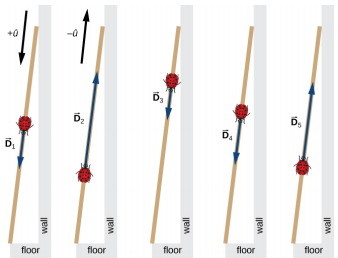— Figure \(\PageIndex{1}\): Five displacements of the ladybug. Note that in this schematic drawing, magnitudes of displacements are not drawn to scale. (credit: modification of work by “Persian Poet Gal”/Wikimedia Commons)

Solution

The resultant of all the displacement vectors is

\[ \begin{align*} \vec{D} &= \vec{D}_{1} + \vec{D}_{2} + \vec{D}_{3} + \vec{D}_{4} + \vec{D}_{5} \\[4pt] &= (15\; cm)( + \hat{u} ) + (56\; cm)( −\hat{u} ) + (3\; cm)( + \hat{u} ) + (25\; cm)( + \hat{u}) + (19\; cm)( − \hat{u}) \\[4pt] &= (15 − 56 + 3 + 25 − 19) cm\; \hat{u} \\[4pt] &= −32\; cm\; \hat{u} \ldotp \end{align*}\]

In this calculation, we use the distributive law given by Equation 2.2.9. The result reads that the total displacement vector points away from the 100-cm mark (initial landing site) toward the end of the meter stick that touches the wall. The end that touches the wall is marked 0 cm, so the final position of the ladybug is at the (100 – 32) cm = 68-cm mark.

Algebra of Vectors in Two Dimensions

When vectors lie in a plane—that is, when they are in two dimensions—they can be multiplied by scalars, added to other vectors, or subtracted from other vectors in accordance with the general laws expressed by Equation 2.2.1, Equation 2..2.2, Equation 2.2.7, and Equation 2.2.8. However, the addition rule for two vectors in a plane becomes more complicated than the rule for vector addition in one dimension. We have to use the laws of geometry to construct resultant vectors, followed by trigonometry to find vector magnitudes and directions. This geometric approach is commonly used in navigation (Figure \(\PageIndex{2}\)). In this section, we need to have at hand two rulers, a triangle, a protractor, a pencil, and an eraser for drawing vectors to scale by geometric constructions.

A photograph of someone measuring distance on a map using calipers and a ruler. — Figure \(\PageIndex{2}\): In navigation, the laws of geometry are used to draw resultant displacements on nautical maps.

For a geometric construction of the sum of two vectors in a plane, we follow the parallelogram rule. Suppose two vectors \(\vec{A}\) and \(\vec{B}\) are at the arbitrary positions shown in Figure \(\PageIndex{3}\). Translate either one of them in parallel to the beginning of the other vector, so that after the translation, both vectors have their origins at the same point. Now, at the end of vector \(\vec{A}\) we draw a line parallel to vector \(\vec{B}\) and at the end of vector \(\vec{B}\) we draw a line parallel to vector \(\vec{A}\) (the dashed lines in Figure \(\PageIndex{3}\)). In this way, we obtain a parallelogram. From the origin of the two vectors we draw a diagonal that is the resultant \(\vec{R}\) of the two vectors: \(\vec{R}\) = \(\vec{A}\) + \(\vec{B}\) (Figure \(\PageIndex{3a}\)). The other diagonal of this parallelogram is the vector difference of the two vectors \(\vec{D}\) = \(\vec{A}\) − \(\vec{B}\), as shown in Figure \(\PageIndex{3b}\). Notice that the end of the difference vector is placed at the end of vector \(\vec{A}\).

The parallelogram method for adding vectors is illustrated. In figure a, vectors A and B are shown. Vector A points to the right and down and vector B points right and up. Vectors A and B are then shown as solid arrows with their tails together, and their directions as before. A dashed line parallel to vector A but shifted so it starts at the head of B is shown. A second dashed line, parallel to B and starting at the head of A is also shown. The vectors A and B and the two dashed lines form a parallelogram. A third vector, labeled vector R = vector A plus vector B, is shown. The tail of vector R is at the tails of vectors A and B, and the head of vector R is where the dashed lines meet each other, diagonally across the parallelogram. We note that the magnitude of R is not equal to the magnitude of A plus the magnitude of B. In figure b, vectors A and minus B are shown. Vector minus B is vector B from part a, rotated 180 degrees. Vector A points to the right and down and vector minus B points left and down. Vectors A and B are then shown as solid arrows with their tails together, and their directions as before. A dashed line parallel to vector A but shifted so it starts at the head of B is shown. A second dashed line, parallel to B and starting at the head of A is also shown. The vectors A and B and the two dashed lines form a parallelogram. A third vector, labeled vector D is shown. The tail of vector D is at the head of vector B, and the head of vector D is at the head of vector A, diagonally across the parallelogram. We note that vector D is equal to vector A minus vector B, but the magnitude of D is not equal to the magnitude of A minus the B. — Figure \(\PageIndex{3}\): The parallelogram rule for the addition of two vectors. Make the parallel translation of each vector to a point where their origins (marked by the dot) coincide and construct a parallelogram with two sides on the vectors and the other two sides (indicated by dashed lines) parallel to the vectors. (a) Draw the resultant vector \(\vec{R}\) along the diagonal of the parallelogram from the common point to the opposite corner. Length R of the resultant vector is not equal to the sum of the magnitudes of the two vectors. (b) Draw the difference vector \(\vec{D}\) = \(\vec{A}\) − \(\vec{B}\) along the diagonal connecting the ends of the vectors. Place the origin of vector \(\vec{D}\) at the end of vector \(\vec{B}\) and the end (arrowhead) of vector \(\vec{D}\) at the end of vector \(\vec{A}\). Length D of the difference vector is not equal to the difference of magnitudes of the two vectors.

It follows from the parallelogram rule that neither the magnitude of the resultant vector nor the magnitude of the difference vector can be expressed as a simple sum or difference of magnitudes A and B, because the length of a diagonal cannot be expressed as a simple sum of side lengths. When using a geometric construction to find magnitudes |\(\vec{R}\)| and |\(\vec{D}\)|, we have to use trigonometry laws for triangles, which may lead to complicated algebra. There are two ways to circumvent this algebraic complexity. One way is to use the method of components, which we examine in the next section. The other way is to draw the vectors to scale, as is done in navigation, and read approximate vector lengths and angles (directions) from the graphs. In this section we examine the second approach.

If we need to add three or more vectors, we repeat the parallelogram rule for the pairs of vectors until we find the resultant of all of the resultants. For three vectors, for example, we first find the resultant of vector 1 and vector 2, and then we find the resultant of this resultant and vector 3. The order in which we select the pairs of vectors does not matter because the operation of vector addition is commutative and associative (see Equation 2.2.7 and Equation 2.2.8). Before we state a general rule that follows from repetitive applications of the parallelogram rule, let’s look at the following example.

Suppose you plan a vacation trip in Florida. Departing from Tallahassee, the state capital, you plan to visit your uncle Joe in Jacksonville, see your cousin Vinny in Daytona Beach, stop for a little fun in Orlando, see a circus performance in Tampa, and visit the University of Florida in Gainesville. Your route may be represented by five displacement vectors \(\vec{A}\), \(\vec{B}\), \(\vec{C}\), \(\vec{D}\), and \(\vec{E}\), which are indicated by the red vectors in Figure \(\PageIndex{4}\). What is your total displacement when you reach Gainesville? The total displacement is the vector sum of all five displacement vectors, which may be found by using the parallelogram rule four times. Alternatively, recall that the displacement vector has its beginning at the initial position (Tallahassee) and its end at the final position (Gainesville), so the total displacement vector can be drawn directly as an arrow connecting Tallahassee with Gainesville (see the green vector in Figure \(\PageIndex{4}\)). When we use the parallelogram rule four times, the resultant \(\vec{R}\) we obtain is exactly this green vector connecting Tallahassee with Gainesville: \(\vec{R}\) = \(\vec{A}\) + \(\vec{B}\) + \(\vec{C}\) + \(\vec{D}\) + \(\vec{E}\).

A map of Florida with the following vectors shown in red: Vector A from Tallahassee to Jacksonville, almost due west. Vector B from Jacksonville to Daytona Beach, southeast. Vector C from Daytona Beach to Orlando, southwest. Vector D from Orlando to Tampa, southwest (but less vertical than vector C). Vector E from Tampa to Gainesville, slightly east of north. Vector R from Tallahassee to Gainsville is shown as a green arrow. — Figure \(\PageIndex{4}\): When we use the parallelogram rule four times, we obtain the resultant vector \(\vec{R}\) = \(\vec{A}\) + \(\vec{B}\) + \(\vec{C}\) + \(\vec{D}\) + \(\vec{E}\), which is the green vector connecting Tallahassee with Gainesville.

Drawing the resultant vector of many vectors can be generalized by using the following tail-to-head geometric construction. Suppose we want to draw the resultant vector \(\vec{R}\) of four vectors \(\vec{A}\), \(\vec{B}\), \(\vec{C}\), and \(\vec{D}\) (Figure \(\PageIndex{5a}\)). We select any one of the vectors as the first vector and make a parallel translation of a second vector to a position where the origin (“tail”) of the second vector coincides with the end (“head”) of the first vector. Then, we select a third vector and make a parallel translation of the third vector to a position where the origin of the third vector coincides with the end of the second vector. We repeat this procedure until all the vectors are in a head-to-tail arrangement like the one shown in Figure \(\PageIndex{5}\). We draw the resultant vector \(\vec{R}\) by connecting the origin (“tail”) of the first vector with the end (“head”) of the last vector. The end of the resultant vector is at the end of the last vector. Because the addition of vectors is associative and commutative, we obtain the same resultant vector regardless of which vector we choose to be first, second, third, or fourth in this construction.

In figure a, four vectors, labeled A, B, C, and D are shown individually. In figure b, the vectors are shown arranged head to tail: Vector A’s tail is at the head of D. Vector C’s tail is at the head of A. And vector B’s tail is at the head of C. Each vector is pointing in the same direction as it is in figure a. A fifth vector, R, starts at the tail of vector D and ends at the head of vector B. — Figure \(\PageIndex{5}\): Tail-to-head method for drawing the resultant vector \(\vec{R}\) = \(\vec{A}\) + \(\vec{B}\) + \(\vec{C}\) + \(\vec{D}\). (a) Four vectors of different magnitudes and directions. (b) Vectors in (a) are translated to new positions where the origin (“tail”) of one vector is at the end (“head”) of another vector. The resultant vector is drawn from the origin (“tail”) of the first vector to the end (“head”) of the last vector in this arrangement.

Example \(\PageIndex{2}\): Geometric Construction of the Resultant

The three displacement vectors \(\vec{A}\), \(\vec{B}\), and \(\vec{C}\) in Figure \(\PageIndex{6}\) are specified by their magnitudes A = 10.0, B = 7.0, and C = 8.0, respectively, and by their respective direction angles with the horizontal direction \(\alpha\) = 35°, \(\beta\) = −110°, and \(\gamma\) = 30°. The physical units of the magnitudes are centimeters. Choose a convenient scale and use a ruler and a protractor to find the following vector sums: (a) \(\vec{R}\) = \(\vec{A}\) + \(\vec{B}\), (b) \(\vec{D}\) = \(\vec{A}\) − \(\vec{B}\), and (c) \(\vec{S}\) = \(\vec{A}\) − \(3 \vec{B}\) + \(\vec{C}\).

Vector A has magnitude 10.0 and is at an angle alpha = 35 degrees counterclockwise from the horizontal. It points up and right. Vector B has magnitude 7.0 and is at an angle beta = -110 degrees clockwise from the horizontal. It points down and left. Vector C has magnitude 8.0 and is at an angle gamma = 30 degrees counterclockwise from the horizontal. It points up and right. Vector F has magnitude 20.0 and is at an angle phi = 110 degrees counterclockwise from the horizontal. It points up and left. — Figure \(\PageIndex{6}\): Vectors used in Example \(\PageIndex{2}\) and in the Exercise feature that follows.

Strategy

In geometric construction, to find a vector means to find its magnitude and its direction angle with the horizontal direction. The strategy is to draw to scale the vectors that appear on the right-hand side of the equation and construct the resultant vector. Then, use a ruler and a protractor to read the magnitude of the resultant and the direction angle. For parts (a) and (b) we use the parallelogram rule. For (c) we use the tail-to-head method.

Solution

For parts (a) and (b), we attach the origin of vector \(\vec{B}\) to the origin of vector \(\vec{A}\), as shown in Figure \(\PageIndex{7}\), and construct a parallelogram. The shorter diagonal of this parallelogram is the sum \(\vec{A}\) + \(\vec{B}\). The longer of the diagonals is the difference \(\vec{A}\) − \(\vec{B}\). We use a ruler to measure the lengths of the diagonals, and a protractor to measure the angles with the horizontal. For the resultant \(\vec{R}\), we obtain R = 5.8 cm and \(\theta_{R}\) ≈ 0°. For the difference \(\vec{D}\), we obtain D = 16.2 cm and \(\theta_{D}\) = 49.3°, which are shown in Figure \(\PageIndex{7}\).

Three diagrams of vectors A and B. Vectors A and B are shown placed tail to tail. Vector A points up and right and has magnitude 10.0. Vector B points down and left and has magnitude 7.0. The angle between vectors A and B is 145 degrees. In the second diagram, Vectors A and B are shown again along with the dashed lines completing the parallelogram. Vector R equaling the sum of vectors A and B is shown as the vector from the tails of A and B to the opposite vertex of the parallelogram. The magnitude of R is 5.8. In the third diagram, Vectors A and B are shown again along with the dashed lines completing the parallelogram. Vector D equaling the difference of vectors A and B is shown as the vector from the head of B to the head of A. The magnitude of D is 16.2, and the angle between D and the horizontal is 49.3 degrees. Vector R in the second diagram is much shorter than vector D in the third diagram. — Figure \(\PageIndex{7}\): Using the parallelogram rule to solve (a) (finding the resultant, red) and (b) (finding the difference, blue).

For (c), we can start with vector −3 \(\vec{B}\) and draw the remaining vectors tail-to-head as shown in Figure \(\PageIndex{8}\). In vector addition, the order in which we draw the vectors is unimportant, but drawing the vectors to scale is very important. Next, we draw vector \(\vec{S}\) from the origin of the first vector to the end of the last vector and place the arrowhead at the end of \(\vec{S}\). We use a ruler to measure the length of \(\vec{S}\), and find that its magnitude is S = 36.9 cm. We use a protractor and find that its direction angle is \(\theta_{S}\) = 52.9°. This solution is shown in Figure \(\PageIndex{8}\).

Three vectors are shown in blue and placed head to tail: Vector minus 3 B points up and right and has magnitude 3 B = 21.0. Vector A starts at the head of B, points up and right, and has a magnitude of A=10.0. The angle between vector A and vector minus 3 B is 145 degrees. Vector C starts at the head of A and has magnitude C=8.0. Vector S is green and goes from the tail of minus 3 B to the head of C. Vector S equals vector A minus 3 vector B plus vector C, has a magnitude of S=36.9 and makes an angle of 52.9 degrees counterclockwise with the horizontal. — Figure \(\PageIndex{8}\): Using the tail-to-head method to solve (c) (finding vector \(\vec{S}\), green).