2.7.26: Further Vector Topics

Vector Basics

Classical mechanics describes the motion of bodies as they move through space. To describe a motion in space it is not sufficient to give a position and a speed: you need a direction as well. Therefore we work with vectors: mathematical objects that have both a magnitude and a direction. If you tell me you’re moving, I know something, but not much; I’ll know more if you tell me you’re moving at walking speed, and have full information of your velocity once you tell me that you’re moving at walking speed towards the coffee machine. Although in principle we could make do with specifying a magnitude and direction of every vector in this way, it is often more convenient to express our vectors in a basis. To do so, we choose an (arbitrary) origin, and as many basis vectors as we have spatial dimensions, in such a way that they are not parallel to one another, and usually mutually perpendicular (orthogonal) and of unit length (orthonormal). Then we decompose our vector by giving its components along each of the basis vectors. The most common choice is to use a Cartesian basis, of two or three (depending on spatial dimension) basis vectors of unit length pointing in the standard x, y and z directions, and indicated as \(\hat{\boldsymbol{x}}, \hat{\boldsymbol{y}}\) and \(\hat{\boldsymbol{z}}\), or (rather annoyingly) sometimes as \(\boldsymbol{i}, \boldsymbol{j}\) and \(\boldsymbol{k}\), the latter especially in American textbooks. Other often encountered systems are polar coordinates (2D) and cylindrical and spherical coordinates (3D), see the mathematical appendix for more background on those. To write our vectors, we now specify the components in each direction, writing for example \(\boldsymbol{v}=3 \hat{\boldsymbol{x}}+3 \hat{\boldsymbol{y}}\) for a vector (in boldface) representing a speed of \(3 \sqrt{2}\) and a direction making an angle of \(45^{\circ}\) with the horizontal.

Vectors can be added and subtracted just like scalars - simply add and subtract them by component. Graphically, you add two vectors by putting them head-to-tail: you can find the sum of two vectors \(\boldsymbol{v}\) and \(\boldsymbol{w}\) by putting the start of \(\boldsymbol{w}\) at the end of \(\boldsymbol{v}\), the sum \(\boldsymbol{v} + \boldsymbol{w}\) then points from the start of \(\boldsymbol{v}\) to the end of \(\boldsymbol{w}\). You can also multiply a vector by a scalar, by multiplying every component of the vector with that scalar. Graphically, this means that you extend the length of the vector with the scalar factor you just multiplied with.

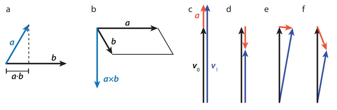
You can’t take the product of two vectors like you would two scalars. There are however two vector operations that closely resemble the product, known as the inner (or dot) and outer (or cross) product, see Figure 16.A.1. The dot product represents the length of the projection of one vector on another (and thus gives a scalar); it is zero for perpendicular vectors, and the dot product of a vector with itself gives the square of its length. To calculate the dot product of two vectors, sum the products of their components: if \(\boldsymbol{v}=v_{x} \hat{\boldsymbol{x}}+v_{y} \hat{\boldsymbol{y}}\) and \(\boldsymbol{w}=w_{x} \hat{\boldsymbol{x}}+w_{y} \hat{y}\), then \(\boldsymbol{v} \cdot \boldsymbol{w}=v_{x} w_{x}+v_{y} w_{y}\). You can use the dot product to find the angle between two vectors, using standard geometry, which gives

\[\cos \theta=\frac{\boldsymbol{v} \cdot \boldsymbol{w}}{|\boldsymbol{v}||\boldsymbol{w}|}=\frac{v_{x} w_{x}+v_{y} w_{y}}{|\boldsymbol{v}||\boldsymbol{w}|}\]

where \(|\boldsymbol{v}|\) and \(|\boldsymbol{w}|\) are the lengths of vectors \(\boldsymbol{v}\) and \(\boldsymbol{w}\), respectively. The cross product is only defined for three-dimensional vectors, say \(\boldsymbol{v}=v_{x} \hat{\boldsymbol{x}}+v_{y} \hat{\boldsymbol{y}}+v_{z} \hat{\boldsymbol{z}}\) and \(\boldsymbol{w}=w_{x} \hat{\boldsymbol{x}}+w_{y} \hat{\boldsymbol{y}}+w_{z} \hat{z}\). The result is another vector, with a direction perpendicular to the plane spanned by \(\boldsymbol{v}\) and \(\boldsymbol{w}\), and a magnitude equal to the area of the parallelogram bounded by them. The cross product is most easily expressed in column vector form:

\[\boldsymbol{v} \times \boldsymbol{w}=\left(\begin{array}{c}
{v_{x}} \\
{v_{y}} \\
{v_{z}}
\end{array}\right) \times\left(\begin{array}{c}
{w_{x}} \\
{w_{y}} \\
{w_{z}}
\end{array}\right)=\left(\begin{array}{c}
{v_{y} w_{z}-v_{z} w_{y}} \\
{v_{z} w_{x}-v_{x} w_{z}} \\
{v_{x} w_{y}-v_{y} w_{x}}
\end{array}\right)\]

The cross product of a vector with itself is zero.

Figure \(\PageIndex{1}\): Products and derivatives of vectors. (a) The dot product of two vectors \(\boldsymbol{a}\) and \(\boldsymbol{b}\) gives the length of the projection of \(\boldsymbol{a}\) on \(\boldsymbol{b}\) (or vice versa). (b) The cross product of two vectors \(\boldsymbol{a}\) and \(\boldsymbol{b}\) gives a vector perpendicular to the plane spanned by \(\boldsymbol{a}\) and \(\boldsymbol{b}\) and with a magnitude equal to the area of the parallelogram spanned by \(\boldsymbol{a}\) and \(\boldsymbol{b}\). (c-f ) Acceleration as a change in velocity. In every panel, the original velocity is shown in black, the velocity a short time ∆t later is shown in blue, and the acceleration is shown in red. (c) Acceleration for an increase in the magnitude of the velocity. (d) Acceleration for a decrease in the magnitude of the velocity. (e) Acceleration for a change in direction of the velocity at constant magnitude. (f ) Acceleration for a change in velocity that involves both a change in direction and a decrease in magnitude.

Vectors can be functions, just like scalar quantities: they can depend on one or more parameters, like position or time. Also, again just like scalar functions, you can calculate a rate of change of vector function as you move through parameter values, for instance asking how the velocity of a car changes as a function of time. An instantaneous rate of change is simply a derivative, which is calculated in exactly the same manner as the derivative of a scalar function. For example, the rate of change of the velocity, known as the acceleration \(\boldsymbol{a}\), is defined as:

\[\boldsymbol{a}=\lim _{\Delta t \rightarrow 0} \frac{\boldsymbol{v}(t+\Delta t)-\boldsymbol{v}}{\Delta t}\]

Since the velocity itself is the derivative of the position \(\boldsymbol{x}(t)\), the acceleration is also the second derivative of the position. Time derivatives occur so frequently in classical mechanics that we use a special notation for them: a first derivative is indicated by a dot on top of the quantity, and a second derivative by a double dot - so we have \(\boldsymbol{a}=\boldsymbol{\dot { x }}=\ddot{\boldsymbol{x}}\).

Vector derivatives are somewhat richer than those of scalar functions, since there are more ways that a vector can change. Like a scalar function, the magnitude of a vector can increase or decrease. Moreover, its direction can also change, which also means that it has a nonzero derivative, and of course, you can have a combination of a change in magnitude and a change in direction, see Figure 16.A.1.

Figure \(\PageIndex{2}\): Examples of scalar and vector fields. (a) Temperature (a scalar) at every point in the Netherlands at 11:30 on October 28, 2013. Lines of equal temperature are drawn in black; the gradient of the temperature field is everywhere perpendicular to these lines. (b) Wind velocity (a vector) at every point in the Netherlands at the same time as the temperature map. Colors correspond to the magnitude of the velocity. (a and b) from [30]. (c) Example of a vector field with a large divergence and zero curl. (d) Example of a vector field with a large curl (and low but nonzero divergence).

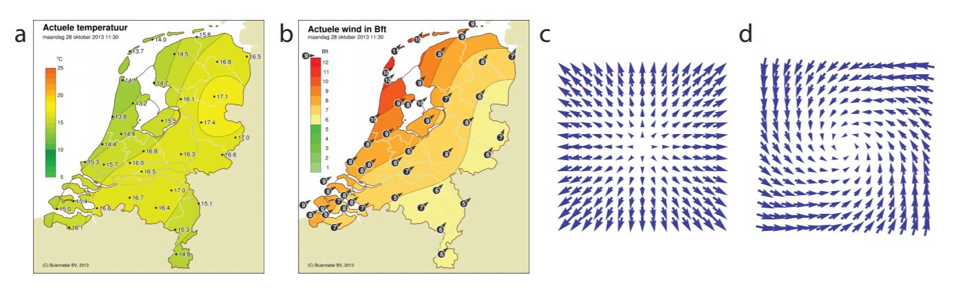
Functions (scalar or vector) that are defined at every point in space are sometimes called fields. Examples are the temperature (scalar) and wind (vector) at every point on the planet, see Figure 16.A.2. Just like you can calculate the rate of change of a function in time, you can also consider how a function changes in space. For a scalar function, this quantity is a vector, known as the gradient, defined as the vector of partial derivatives. For a function f (x, y, z), we have:

\[\boldsymbol{\nabla} f=\frac{\partial f}{\partial x} \hat{\boldsymbol{x}}+\frac{\partial f}{\partial y} \hat{\boldsymbol{y}}+\frac{\partial f}{\partial z} \hat{\boldsymbol{z}}=\left(\begin{array}{c}
{\partial f / \partial x} \\
{\partial f / \partial y} \\
{\partial f / \partial z}
\end{array}\right)\]

The direction of \(\boldsymbol{\nabla} f\) is the direction of maximal change, and its magnitude tells you how quickly the function changes in that direction. For a vector field \(\boldsymbol{v}\), we can’t take the gradient, but we can use the ‘vector’ \(\boldsymbol{\nabla}\) of partial derivatives combined with either the dot or cross product. The first option is known as the divergence of \(\boldsymbol{v}\), and tells you how quickly \(\boldsymbol{v}\) spreads out; the second is the curl of \(\boldsymbol{v}\) and tells you how much \(\boldsymbol{v}\) rotates:

\[\begin{align}
\operatorname{div}(\boldsymbol{v}) &=\boldsymbol{\nabla} \cdot \boldsymbol{v}=\frac{\partial v_{x}}{\partial x}+\frac{\partial v_{y}}{\partial y}+\frac{\partial v_{z}}{\partial z} \\
\operatorname{curl}(\boldsymbol{v}) &=\boldsymbol{\nabla} \times \boldsymbol{v}=\left(\begin{array}{c}
{\partial_{y} v_{z}-\partial_{z} v_{y}} \\
{\partial_{z} v_{x}-\partial_{x} v_{z}} \\
{\partial_{x} v_{y}-\partial_{y} v_{x}}
\end{array}\right)
\end{align}\]

where \(\partial_{x}= \frac{\partial}{\partial x}\), and so on.

Polar Coordinates

You can specify any point in the plane by specifying its projection on two perpendicular axes - we typically call these the x and y-axes and x and y coordinates. In this Cartesian system (named after Descartes), we identify unit vectors \(\hat{\boldsymbol{x}}\) and \(\hat{\boldsymbol{y}}\), pointing along their respective axes, and being of unit length. A position \(\boldsymbol{r}\) can then be decomposed in the two directions: \(\boldsymbol{r}=r_{x} \hat{\boldsymbol{x}}+r_{y} \hat{\boldsymbol{y}}\), with \(r_{x}=\boldsymbol{r} \cdot \hat{\boldsymbol{x}}\) and \(r_{y}=\boldsymbol{r} \cdot \hat{\boldsymbol{y}}\). Alternatively, we can write \(\hat{\boldsymbol{x}}=\left(\begin{array}{l}
{1} \\
{0}
\end{array}\right)\) and \(\hat{\boldsymbol{y}}=\left(\begin{array}{l}
{0} \\
{1}
\end{array}\right)\), which gives for \(\boldsymbol{r}\):

\[\boldsymbol{r}=r_{x} \hat{\boldsymbol{x}}+r_{y} \hat{\boldsymbol{y}}=\left(\begin{array}{l}
{r_{x}} \\
{r_{y}}
\end{array}\right)\]

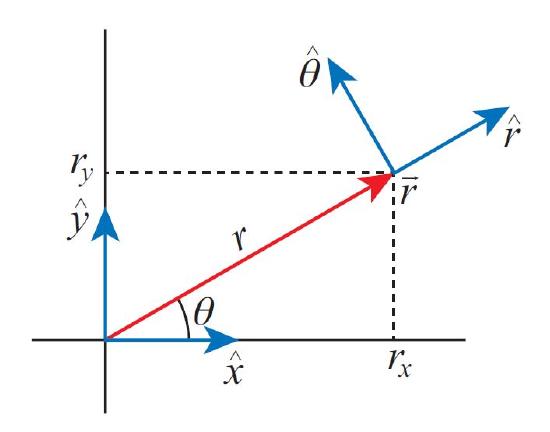
Instead of specifying the x and y coordinates of our position, we could also uniquely identify it by giving two different numbers: its distance to the origin r, and the angle \(\theta\) the line to the origin makes with a fixed reference axis (typically the x-axis), see Figure 16.A.3. Invoking the Pythagorean theorem and basic trigonometry,
we readily find \(r=\sqrt{r_{x}^{2}+r_{y}^{2}}\) and \(\tan \theta= \frac{r_{y}}{r_{x}}\). We call r the length of the vector \(\boldsymbol{r}\). We could also invert the relations for r and \(\theta\) so we can get the Cartesian components if the length and angle are known: \(r_{x}=r \cos \theta\) and \(r_{y}=r \sin \theta\).

Like the Cartesian basis vectors \(\hat{\boldsymbol{x}}\) and (\hat{\boldsymbol{y}}\), which point in the direction of increasing x and y values, we can also define unit vectors pointing in the direction of increasing r and \(\theta\). These directions do depend on our position in space, but they do have a clear geometrical interpretation: \hat{\boldsymbol{r}} always points radially outward from the origin, and \hat{\boldsymbol{\theta}} in the direction you’d move if you’d be making a counterclockwise rotation about the origin. Given a position vector \(\boldsymbol{r}\), finding the vector in the direction of increasing r is very easy: \(\hat{\boldsymbol{r}}= \boldsymbol{r} / r\). The expression for r in our new polar basis \((\hat{\boldsymbol{r}}, \hat{\boldsymbol{\theta}})\) is almost tautological: \(\boldsymbol{r}=r \hat{\boldsymbol{r}}\).

Relating the polar basis vectors to the Cartesian ones is straightforward. We have:

\[\boldsymbol{r}=r_{x} \hat{\boldsymbol{x}}+r_{y} \hat{\boldsymbol{y}}=r \hat{\boldsymbol{r}}\]

and using \(r_{x}=r \cos \theta, r_{y}=r \sin \theta\) we also have

\[\boldsymbol{r}=r \cos \theta \hat{\boldsymbol{x}}+r \sin \theta \hat{\boldsymbol{y}}\]

We thus find that \(\hat{\boldsymbol{r}}=\cos \theta \hat{\boldsymbol{x}}+\sin \theta \hat{\boldsymbol{y}}\).

For \(\hat{\boldsymbol{\theta}\) we note that to rotate around the origin, the direction of motion needs to be perpendicular to \(\hat{\boldsymbol{r}}\). There are of course two such directions - we pick the sign by demanding that the counterclockwise rotation is positive. This gives \(\hat{\boldsymbol{\theta}}=\left(r_{y} / r\right) \hat{\boldsymbol{x}}-\left(r_{x} / r\right) \hat{\boldsymbol{y}}=\sin \theta \hat{\boldsymbol{x}}-\cos \theta \hat{\boldsymbol{y}}\). Written out as vectors, we have:

\[\hat{\boldsymbol{r}}=\left(\begin{array}{c}
{\cos \theta} \\
{\sin \theta}
\end{array}\right), \quad \hat{\boldsymbol{\theta}}=\left(\begin{array}{c}
{\sin \theta} \\
{-\cos \theta}
\end{array}\right)\]

Note that

\[\hat{\boldsymbol{r}}=\frac{\partial \hat{\boldsymbol{\theta}}}{\partial \theta}, \quad \hat{\boldsymbol{\theta}}=-\frac{\partial \hat{\boldsymbol{r}}}{\partial \theta}\]

Naturally, we can also express the Cartesian basis in terms of the polar ones:

\[\hat{\boldsymbol{x}}=\cos \theta \hat{\boldsymbol{r}}+\sin \theta \hat{\boldsymbol{\theta}}, \quad \hat{\boldsymbol{y}}=\sin \theta \hat{\boldsymbol{r}}-\cos \theta \hat{\boldsymbol{\theta}}\]

Figure \(\PageIndex{3}\): Polar coordinate system and polar unit vectors. A position \(\boldsymbol{r}\) in the plane can be specified either by giving its projections on two reference axes (along the \(\hat{\boldsymbol{x}}\) and \(\hat{\boldsymbol{x}}\) direction), or by giving its distance r to the origin, and the angle \(\theta\) the line to the origin makes with the x axis. The polar basis vectors are defined as pointing in the direction of increasing r (i.e., radially outward), and increasing \(\theta\) (i.e., rotating counterclockwise around the origin).