3.1: Position, Displacement and Distance

Learning Objectives

• Define position, displacement, and distance traveled.
• Calculate the total displacement given the position as a function of time.
• Determine the total distance traveled.

When we discuss motion of an object, we often ask: Where is it? Where is it going? How fast is it getting there? How long did it take it to get there? etc... The answers to these questions and more require that we specify the position, displacement, and time of travel of the object.

Position

To describe the motion of an object, you must first be able to describe its position \(\vec{r}(t)\) where it is at any particular time \(t\). More precisely, we need to specify its position relative to a convenient frame of reference, an arbitrary set of axes from which the position and motion of the object are described. Earth is often used as a frame of reference, and we often describe the position of an object as it relates to stationary objects on Earth. For example, a rocket launch could be described in terms of the position of the rocket with respect to Earth as a whole, whereas a cyclist’s position could be described in terms of where she is in relation to the buildings she passes. In other cases, we use reference frames that are not stationary but are in motion relative to Earth. To describe the position of a person in an airplane, for example, we use the airplane, not Earth, as the reference frame. To describe the position of an object undergoing one dimensional motion, we often use the variable \(x\) if it is moving horizontally and \(y\) if it is moving vertically.

For motion in two and three dimensions, we generally use the coordinates \(x\), \(y\), and \(z\) to locate a particle at point \(P(x, y, z)\). If the particle is moving, the variables \(x\), \(y\), and \(z\) are functions of time (\(t\)):

\[x = x(t) \quad y = y(t) \quad z = z(t) \ldotp \label{4.1}\]

The position vector from the origin of the coordinate system to point P is \(\vec{r}(t)\). In unit vector notation, \(\vec{r}\)(t) is

\[\vec{r} (t) = x(t)\; \hat{i} + y(t)\; \hat{j} + z(t)\; \hat{k} \ldotp \label{4.2}\]

Figure \(\PageIndex{1}\) shows the coordinate system and the vector to point \(P\), where a particle could be located at a particular time \(t\). Note the orientation of the x, y, and z axes. This orientation is called a right-handed coordinate system and it is used throughout the chapter.

Figure \(\PageIndex{1}\): A three-dimensional coordinate system with a particle at position \(P(x(t), y(t), z(t))\).

Displacement

If an object moves relative to a frame of reference, the object’s position changes. This change in position is called displacement. The word displacement implies that an object has moved, or has been displaced. Since displacement indicates direction, it is a vector.

Figure \(\PageIndex{2}\): The displacement \(\Delta \vec{r} = \vec{r}(t_2) − \vec{r}(t_1)\) is the vector from \(P_1\) to \(P_2\).

With our definition of the position of a particle in three-dimensional space, we can formulate the three-dimensional displacement. Figure \(\PageIndex{2}\) shows a particle at time t₁ located at P₁ with position vector \(\vec{r}\)(t₁). At a later time t₂, the particle is located at P₂ with position vector \(\vec{r}\)(t₂). The displacement vector \(\Delta \vec{r}\) is found by subtracting \(\vec{r}(t_1)\) from \(\vec{r}(t_2)\):

\[\Delta \vec{r} = \vec{r} (t_{2}) - \vec{r} (t_{1}) \ldotp \label{4.3}\]

Note that the SI unit for displacement is the meter, but sometimes we use kilometers or other units of length. Keep in mind that when units other than meters are used in a problem, you may need to convert them to meters to complete the calculation.

The following examples illustrate the concept of displacement:

Example 4.1: Polar Orbiting Satellite

A satellite is in a circular polar orbit around Earth at an altitude of 400 km—meaning, it passes directly overhead at the North and South Poles. What is the magnitude and direction of the displacement vector from when it is directly over the North Pole to when it is at −45° latitude?

Strategy

We make a picture of the problem to visualize the solution graphically. This will aid in our understanding of the displacement. We then use unit vectors to solve for the displacement.

Strategy

Figure \(\PageIndex{3}\) shows the surface of Earth and a circle that represents the orbit of the satellite. Although satellites are moving in three-dimensional space, they follow trajectories of ellipses, which can be graphed in two dimensions. The position vectors are drawn from the center of Earth, which we take to be the origin of the coordinate system, with the y-axis as north and the x-axis as east. The vector between them is the displacement of the satellite. We take the radius of Earth as 6370 km, so the length of each position vector is 6770 km.

Figure \(\PageIndex{3}\): Two position vectors are drawn from the center of Earth, which is the origin of the coordinate system, with the y-axis as north and the x-axis as east. The vector between them is the displacement of the satellite.

In unit vector notation, the position vectors are

\[ \begin{align*} \vec{r}(t_{1}) &= 6770 \ldotp \; km\; \hat{j} \\[4pt] \vec{r}(t_{2}) &= 6770 \ldotp \; km (\cos (-45°))\; \hat{i} + 6770 \ldotp \; km (\sin(−45°))\; \hat{j} \ldotp \end{align*}\]

Evaluating the sine and cosine, we have

\[ \begin{align*} \vec{r}(t_{1}) &= 6770 \ldotp \hat{j} \\[4pt] \vec{r}(t_{2}) &= 4787\; \hat{i} − 4787\; \hat{j} \ldotp \end{align*}\]

Now we can find \(\Delta \vec{r}\), the displacement of the satellite:

\[\Delta \vec{r} = \vec{r} (t_{2}) - \vec{r} (t_{1}) = 4787\; \hat{i} - 11,557\; \hat{j} \ldotp \nonumber\]

The magnitude of the displacement is

\[|\Delta \vec{r}| = \sqrt{(4787)^{2} + (-11,557)^{2}} = 12,509\; km. \nonumber\]

The angle the displacement makes with the x-axis is

\[\theta = \tan^{-1} \left(\dfrac{-11,557}{4787}\right) = -67.5^{o} \nonumber.\]

Significance

Plotting the displacement gives information and meaning to the unit vector solution to the problem. When plotting the displacement, we need to include its components as well as its magnitude and the angle it makes with a chosen axis—in this case, the x-axis (Figure \(\PageIndex{4}\)).

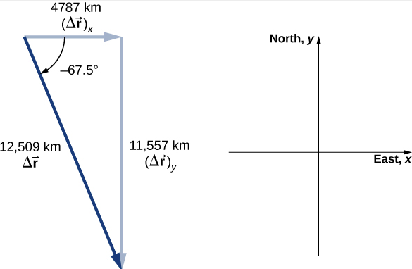
Figure \(\PageIndex{4}\): Displacement vector with components, angle, and magnitude.

Note that the satellite took a curved path along its circular orbit to get from its initial position to its final position in this example. It also could have traveled 4787 km east, then 11,557 km south to arrive at the same location. Both of these paths are longer than the length of the displacement vector. In fact, the displacement vector gives the shortest path between two points in one, two, or three dimensions.

Many applications in physics can have a series of displacements, as discussed in the previous chapter. The total displacement is the sum of the individual displacements, only this time, we need to be careful, because we are adding vectors. We illustrate this concept with an example of Brownian motion.

Example 4.2: Brownian Motion

Brownian motion is a chaotic random motion of particles suspended in a fluid, resulting from collisions with the molecules of the fluid. This motion is three-dimensional. The displacements in numerical order of a particle undergoing Brownian motion could look like the following, in micrometers (Figure \(\PageIndex{5}\)):

\[\Delta \vec{r}_{1} = 2.0\; \hat{i} + \hat{j} + 3.0 \hat{k}\]

\[\Delta \vec{r}_{2} = - \hat{i} + 3.0\; \hat{k}\]

\[\Delta \vec{r}_{3} = 4.0\; \hat{i} -2.0\; \hat{j} + \hat{k}\]

\[\Delta \vec{r}_{4} = -3.0\; \hat{i} + \hat{j} + 3.0\; \hat{k} \ldotp\]

What is the total displacement of the particle from the origin?

Figure \(\PageIndex{5}\): Trajectory of a particle undergoing random displacements of Brownian motion. The total displacement is shown in red.

Solution

We form the sum of the displacements and add them as vectors:

\[\begin{split} \Delta \vec{r}_{Total} & = \sum \Delta \vec{r}_{i} = \Delta \vec{r}_{1} + \Delta \vec{r}_{2} + \Delta \vec{r}_{3} + \Delta \vec{r}_{4} \\ & = (2.0 - 1.0 + 4.0 - 3.0)\; \hat{i} + (1.0 + 0 - 2.0 + 1.0)\; \hat{j} + (3.0 +3.0 + 1.0 + 2.0)\; \hat{k} \\ & = 2.0\; \hat{i} + 0\; \hat{j} + 9.0\; \hat{k}\; \mu m \ldotp \end{split}\]

To complete the solution, we express the displacement as a magnitude and direction,

\[| \Delta \vec{r}_{Total}| = \sqrt{2.0^{2} + 0^{2} + 9.0^{2}} = 9.2 \mu m, \quad \theta = \tan^{-1} \left(\dfrac{9}{2}\right) = 77^{o},\]

with respect to the x-axis in the xz-plane.

Significance

From the figure we can see the magnitude of the total displacement is less than the sum of the magnitudes of the individual displacements.

Displacement in One Dimension

If an object moves along a straight line—for example, if a professor moves to the right relative to a whiteboard Figure \(\PageIndex{3}\)— as mentioned earlier, we often use the variable \(x\) to provide its position if it is moving horizontally and \(y\) if it is moving vertically. The displacement is still a vector. However, we normally just use the sign to indicate direction.

Figure \(\PageIndex{3}\): A professor paces left and right while lecturing. Her position relative to Earth is given by x. The +2.0-m displacement of the professor relative to Earth is represented by an arrow pointing to the right.

Displacement along \(x\)

Displacement \(\Delta x\) is the change in position of an object:

\[\Delta x = x_{f} - x_{0}, \label{3.1}\]

where \(\Delta x\) is the displacement, \(x_{f}\) is the final position, and \(x_{0}\) is the initial position.

Objects in motion can also have a series of displacements. In the previous example of the pacing professor, the individual displacements are 2 m and −4 m, giving a total displacement of −2 m. We define total displacement \(\Delta\)x_Total, as the sum of the individual displacements, and express this mathematically with the equation

\[\Delta x_{Total} = \sum \Delta x_{i}, \label{3.2}\]

where \(\delta\)x_i are the individual displacements. In the earlier example,

\[\Delta x_{1} = x_{1} - x_{0} = 2 - 0 = 2\; m \ldotp\]

Similarly,

\[\Delta x_{2} = x_{2} - x_{1} = -2 - (2) = -4 \; m \ldotp\]

Thus,

\[\Delta x_{total} = x_{1} + x_{2} = 2 - 4 = -2\; m \ldotp\]

The total displacement is 2 − 4 = −2 m to the left, or in the negative direction. It is also useful to calculate the magnitude of the displacement, or its size. The magnitude of the displacement is always positive. This is the absolute value of the displacement, because displacement is a vector and cannot have a negative value of magnitude. In our example, the magnitude of the total displacement is 2 m, whereas the magnitudes of the individual displacements are 2 m and 4 m.

The magnitude of the total displacement should not be confused with the distance traveled. Distance traveled \(x_{total}\)_l, is the total length of the path traveled between two positions. In the previous problem, the distance traveled is the sum of the magnitudes of the individual displacements:

\[x_{total} = |x_{1}| + |x_{2}| = 2 + 4 = 6\; m \ldotp\]