7.5: Center of Mass of Continuous Objects

Learning Objectives

• Explain the meaning and usefulness of the concept of center of mass
• Calculate the center of mass of a given system
• Apply the center of mass concept in two and three dimensions
• Calculate the velocity and acceleration of the center of mass

The center of mass for a continuous object

We now turn to the problem of computing the position of the center of mass of an object whose distribution of mass is known. What follows is pure math, but it is important math that returns over and over in physics.

We will keep this simple by restricting ourselves to objects for which the position of the center of mass in two of the three dimensions is obvious. A good model for this is a simple thin, cylindrical rod. This rod's mass distribution is completely cylindrically symmetric, which means that the center of mass lies on the axis passing through its center. But the mass distribution as a function of position on this axis may not be uniform. For example, it may be more dense on one end than on the other. Put another way, the particles located within the rod may be packed together more tightly in one region of the rod than in another, which means that the center of mass will not necessarily lie at the point halfway between the ends.

We need to say a few words about mass density before we proceed. Density is a measure of how closely-packed in space a quantity of something is. This quantity can be many different things. Here we will be considering mass, but in later physics classes you will deal with density of electric charge (and even, bizarrely, probability!). A uniform density for a region in space means that the quantity (whatever it happens to be) is evenly-distributed everywhere within that region. The way we define an average density for a region in space is to add up how much "stuff" is there, and then divide it by the total space it occupies. This gives an average density, but of course densities can vary from one point in space to another, in which case a density function is defined. We will deal with only the simplest variable densities here. As we will mainly be looking at thin rods for our examples, we will only consider densities that might vary along the length of the rod – this simplifies the process to a single dimension.

The mass density function in this case is a function of a single variable, has units of \(kg/m\), and is called a linear mass density. This mass density function is typically denoted as \(\lambda\left(x\right)\). If it is uniform, then the function is a constant \(\lambda\), and the amount of mass \(m\) within a given length \(l\) is simply given by:

\[ m = \lambda l \]

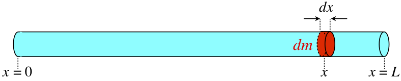
If the density is not uniform, then it is only a constant over an infinitesimal length \(dx\), so that Equation (7.5.1) can only apply to a tiny piece of mass \(dm\), and the relationship is different at every position \(x\) because the density is different at every position:

\[ dm = \lambda \left(x\right) dx \]

Now that we can write down how much mass is at every position, we are ready to do our calculation. We begin by drawing a diagram with the rod in a coordinate system along the \(x\)-axis such that one end is at the origin and the other is at \(x=L\). The Figure below provides a fully-labeled diagram that is very helpful for solving such problems.

Figure \(\PageIndex{1}\)  – Setup Diagram for Computations Involving Mass Density of a Thin Rod.

 

The center of mass is found by multiplying the amount of mass at each point by the \(x\)-coordinate of that mass, then adding up all of those products and dividing by the total mass. Of course, in this case we have an infinite number of point masses, so the sum is infinitely long, but the masses are infinitesimally small, so we solve this by converting the sum into an integral, in which we add up all the pieces from \(x=0\) to \(x=L\):

\[ x_{cm} = \dfrac{dm_1x_1 + dm_2x_2 + \dots}{dm_1 + dm_2 + \dots} = \dfrac{\int\limits_{x=0}^{x=L} dm\;x}{\int\limits_{x=0}^{x=L} dm} \]

Now we plug in Equation (7.5.3) to give the following formula for center of mass (in one dimension) for a thin rod with a linear mass density that varies with \(x\):

\[ x_{cm} = \dfrac{ \displaystyle \int\limits_{x=0}^{x=L} \lambda\left(x\right)xdx}{ \displaystyle \int\limits_{x=0}^{x=L} \lambda\left(x\right)dx} \]

In general, for a continuous object, the position of the center of mass is given by:

 

\[\begin{aligned} \vec r_{CM}=\frac{1}{M}\int \vec r dm\end{aligned}\]

 

\[\therefore \vec r_{CM} = x_{CM} \hat i + y_{CM} \hat j + z_{CM} \hat k = \frac{1}{M} \int x dm \hat i + \frac{1}{M} \int y dm \hat j + \frac{1}{M} \int z dm \hat k\]

where in general, one will need to write \(dm\) in terms of something that depends on position (or a constant) so that the integrals can be evaluated over the spatial coordinates (\(x\),\(y\),\(z\)) over the range that describe the object. In the above, we wrote \(dm = \lambda dx\) to express the mass element in terms of spatial coordinates.

Examples

Example \(\PageIndex{1}\): CM of a Rod of Uniform Mass Density

Find the center of mass of a uniform rod of mass \(M\) and length \(L\).

Solution

If the rod is uniform, then the density is a constant (which we will call simply \(\lambda\)):

\[ x_{cm} = \dfrac{\displaystyle \int \limits_{x=0}^{x=L} \lambda x\,dx}{\displaystyle \int\limits_{x=0}^{x=L} \lambda \,dx} = \dfrac{\cancel{\lambda} \displaystyle \int\limits_{x=0}^{x=L} x\,dx}{\cancel{\lambda} \displaystyle \int\limits_{x=0}^{x=L} dx} = \dfrac{\left[\frac{1}{2}x^2\right]_0^L}{\left[x\right]_0^L}=\frac{1}{2}L\]

So we have calculated what we already knew – that for a thin rod with a uniform mass density, the center of mass is at its center (which on our coordinate system lies at \(L/2\)).

Example \(\PageIndex{1}\): CM of a Rod of Non-Uniform Mass Density

Find the center of mass of a rod of mass \(M\) and length \(L\)and whose mass density varies from one end to the other according to this density function:

\[ \lambda\left(x\right) = \lambda_o\left(\dfrac{x}{L}+1\right)\]

Solution

Before we do the math, let's try to make sense of this function. The easiest way to do this is to consider the endpoints. At \(x=0\), the density equals the constant \(\lambda_o\), while at \(x=L\) that density has grown to twice that much. This increase of density happens linearly with the variable \(x\). What should we expect to see when we compute the center of mass? Well, the rod is more dense near the \(x=L\) end than the \(x=0\) end, so the center of mass should be at an \(x\) value greater than \(L/2\).

\[ x_{cm} = \dfrac{\displaystyle \int\limits_{x=0}^{x=L} \left[\lambda_o\left(\dfrac{x}{L}+1\right)\right]x \,dx}{ \displaystyle \int\limits_{x=0}^{x=L} \left[\lambda_o\left(\dfrac{x}{L}+1\right)\right]dx} = \dfrac{ \displaystyle \cancel{\lambda_o}\int\limits_{x=0}^{x=L} \left(\dfrac{x^2}{L}+x\right)dx}{ \displaystyle \cancel{\lambda_o}\int\limits_{x=0}^{x=L}\left(\dfrac{x}{L}+1\right)dx} = \dfrac{\left[\dfrac{x^3}{3L}+\dfrac{x^2}{2}\right]_0^L}{\left[\dfrac{x^2}{2L}+x\right]_0^L}=\frac{5}{9}L\]

Interestingly, the center of mass doesn't depend upon the density constant \(\lambda_o\).

Example \(\PageIndex{1}\): CM of a Rod of Non-Uniform Mass Density 2

Find the center of mass of a rod of mass \(M\) and length \(L\)and whose mass density varies from one end to the other according to this density function:

\[\begin{aligned} \lambda(x) = 2a + 3bx\end{aligned}\]

Solution

We can still find the center of mass by considering an infinitesimally small mass element of mass \(dm\), and length \(dx\). In terms of the linear mass density and length of the mass element, \(dx\), the mass \(dm\) is given by:

\[\begin{aligned} dm = \lambda(x) dx\end{aligned}\]

The \(x\) position of the center of mass is thus found the same way as before, except that the linear mass density is now a function of \(x\):

\[\begin{aligned} x_{CM} &= \frac{1}{M} \int_0^L \lambda(x) x dx =\frac{1}{M} \int_0^L (2a + 3bx) x dx=\frac{1}{M} \int_0^L (2ax + 3bx^2) dx\\[4pt] &=\frac{1}{M} \left[ ax^2 + bx^3 \right]_0^L\\[4pt] &=\frac{1}{M} (aL^2 + bL^3 )\end{aligned}\]

Example \(\PageIndex{1}\): CM of a Uniform Thin Hoop

Find the center of mass of a uniform thin hoop (or ring) of mass \(M\) and radius \(r\).

Strategy

First, the hoop’s symmetry suggests the center of mass should be at its geometric center. If we define our coordinate system such that the origin is located at the center of the hoop, the integral should evaluate to zero.

We replace dm with an expression involving the density of the hoop and the radius of the hoop. We then have an expression we can actually integrate. Since the hoop is described as “thin,” we treat it as a one-dimensional object, neglecting the thickness of the hoop. Therefore, its density is expressed as the number of kilograms of material per meter. Such a density is called a linear mass density, and is given the symbol \(\lambda\); this is the Greek letter “lambda,” which is the equivalent of the English letter “l” (for “linear”).

Since the hoop is described as uniform, this means that the linear mass density \(\lambda\) is constant. Thus, to get our expression for the differential mass element dm, we multiply \(\lambda\) by a differential length of the hoop, substitute, and integrate (with appropriate limits for the definite integral).

Solution

First, define our coordinate system and the relevant variables (Figure \(\PageIndex{1}\)).

Figure \(\PageIndex{1}\): Finding the center of mass of a uniform hoop. We express the coordinates of a differential piece of the hoop, and then integrate around the hoop.

The center of mass is calculated with Equation \ref{9.34}:

\[\vec{r}_{CM} = \frac{1}{M} \int_{a}^{b} \vec{r} dm \ldotp\]

We have to determine the limits of integration a and b. Expressing \(\vec{r}\) in component form gives us

\[\vec{r}_{CM} = \frac{1}{M} \int_{a}^{b} \big[ (r \cos \theta) \hat{i} + (R \sin \theta) \hat{j} \big] dm \ldotp\]

In the diagram, we highlighted a piece of the hoop that is of differential length ds; it therefore has a differential mass dm = \(\lambda\)ds. Substituting:

\[\vec{r}_{CM} = \frac{1}{M} \int_{a}^{b} \big[ (r \cos \theta) \hat{i} + (R \sin \theta) \hat{j} \big] \lambda ds \ldotp\]

However, the arc length ds subtends a differential angle d\(theta\), so we have

\[ds = rd \theta\]

and thus

\[\vec{r}_{CM} = \frac{1}{M} \int_{a}^{b} \big[ (r \cos \theta) \hat{i} + (R \sin \theta) \hat{j} \big] \lambda rd \theta \ldotp\]

One more step: Since \(\lambda\) is the linear mass density, it is computed by dividing the total mass by the length of the hoop:

\[\lambda = \frac{M}{2 \pi r}\]

giving us

\[\begin{split} \vec{r}_{CM} & = \frac{1}{M} \int_{a}^{b} \big[ (r \cos \theta) \hat{i} + (R \sin \theta) \hat{j} \big] \left(\dfrac{M}{2 \pi r}\right) rd \theta \\ & = \frac{1}{2 \pi} \int_{a}^{b} \big[ (r \cos \theta) \hat{i} + (R \sin \theta) \hat{j} \big] d \theta \ldotp \end{split}\]

Notice that the variable of integration is now the angle \(\theta\). This tells us that the limits of integration (around the circular hoop) are θ = 0 to \(\theta\) = 2\(\pi\), so a = 0 and b = 2\(\pi\). Also, for convenience, we separate the integral into the x- and y-components of \(\vec{r}_{CM}\). The final integral expression is

\[\begin{split} \vec{r}_{CM} & = r_{CM,x} \hat{i} + r_{CM,y} \hat{j} \\ & = \Big[ \frac{1}{2 \pi} \int_{0}^{2 \pi} (2 \cos \theta d \theta \Big] \hat{i} + \Big[ \frac{1}{2 \pi} \int_{0}^{2 \pi} (2 \sin \theta d \theta \Big] \hat{j} \\ & = 0 \hat{i} + 0 \hat{j} = \vec{0} \end{split}\]

as expected.

Example \(\PageIndex{3}\)

Figure \(\PageIndex{5}\): A symmetric bowl with parabolic sides is completely filled with water. The bowl has a height \(h\).

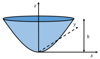
A bowl of height \(h\) has parabolic sides and a circular cross-section, as illustrated in Figure \(\PageIndex{5}\). The bowl is filled with water. The bowl itself has a negligible mass and thickness, so that the mass of the full bowl is dominated by the mass of the water. Where is the center of mass of the full bowl?

Solution

We can define a coordinate system such that the origin is located at the bottom of the bowl and the \(z\) axis corresponds to the axis of symmetry of the bowl. Because the bowl is full of water, and the bowl itself has negligible mass, we can model the full bowl as a uniform body of water with the same shape as the bowl and (volume) mass density \(\rho\) equal to the density of water. Furthermore, by symmetry, the center of mass of the bowl will be on the \(z\) axis.

Because the bowl has a circular cross-section, we can divide it up into disk-shaped mass elements, \(dm\), that have an infinitesimally small height \(dz\), and a radius \(r(z)\), that depends on their \(z\) coordinate (Figure \(\PageIndex{5}\)).

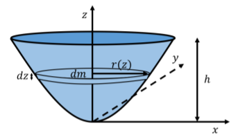
Figure \(\PageIndex{6}\): The parabolic bowl divided up into disk-shaped mass elements, \(dm\), that have an infinitesimally small height \(dz\), and a radius \(r(z)\), that depends on their \(z\) coordinate.

The center of mass of each disk-shaped mass element will be located where the corresponding disk intersects the \(z\) axis. The mass of one disk element is given by:

 

\[\begin{aligned} dm = \rho dV = \rho \pi r^2(z) dz\end{aligned}\]

where \(dV = \pi r(z)^2 dz\) is the volume of the disk with radius \(r(z)\) and thickness \(dz\). The radius of the infinitesimal disk depends on its \(z\) position, since the radii of the different disks must describe a parabola:

\[\begin{aligned} z(r) &= \frac{1}{a^2}r^2\\[4pt] r(z) &= a\sqrt z\\[4pt] \therefore dm &= \rho \pi r^2(z) dz= \rho \pi a^2 z dz\end{aligned}\]

where we introduced the constant \(a\) so that the dimensions are correct. The constant \(a\) determines how “steep” the parabolic sides are. The \(z\) coordinate of the center of mass is thus given by:

\[\begin{aligned} z_{CM} &= \frac{1}{M}\int z dm =\frac{1}{M}\int_0^h z (\rho \pi a^2 z dz)=\frac{\rho \pi a^2}{M}\int_0^h z^2dz \\[4pt] &=\frac{\rho \pi a^2}{M}\left[ \frac{1}{3}z^3 \right]_0^h\\[4pt] &=\frac{\rho \pi a^2}{3M}h^3\end{aligned}\]

However, we are not quite done, since we do not know the total mass, \(M\), of the water. To find the total mass of water, \(M\), we proceed in an analogous way, and determine the value of the sum (integral) of all of the mass elements:

\[\begin{aligned} M = \int dm = \int_0^h \rho \pi a^2 z dz = \rho \pi a^2 \left[ \frac{1}{2}z^2 \right]_0^h= \frac{1}{2}\rho \pi a^2 h^2\end{aligned}\]

Substituting this value for \(M\), we can determine the \(z\) coordinate of the center of mass of the full bowl:

\[\begin{aligned} z_{CM} &=\frac{\rho \pi a^2}{3M}h^3 = \frac{2\rho \pi a^2}{3\rho \pi a^2 h^2}h^3=\frac{2}{3}h\end{aligned}\]

Regardless of the actual shape of the parabola (the parameter \(a\)), the center of mass will always be two thirds of the way up from the bottom of the bowl.

Discussion

In determining the center of mass of a three dimensional object, we used symmetry to argue that the \(x\) and \(y\) coordinates would be zero. We then found the \(z\) position of the center of mass by dividing up the bowl into infinitesimally small mass elements (disks) along the direction in which we needed to find the center of mass coordinate.