11.2: Mathematics of Waves
- Page ID
- 68850
\( \newcommand{\vecs}[1]{\overset { \scriptstyle \rightharpoonup} {\mathbf{#1}} } \)
\( \newcommand{\vecd}[1]{\overset{-\!-\!\rightharpoonup}{\vphantom{a}\smash {#1}}} \)
\( \newcommand{\dsum}{\displaystyle\sum\limits} \)
\( \newcommand{\dint}{\displaystyle\int\limits} \)
\( \newcommand{\dlim}{\displaystyle\lim\limits} \)
\( \newcommand{\id}{\mathrm{id}}\) \( \newcommand{\Span}{\mathrm{span}}\)
( \newcommand{\kernel}{\mathrm{null}\,}\) \( \newcommand{\range}{\mathrm{range}\,}\)
\( \newcommand{\RealPart}{\mathrm{Re}}\) \( \newcommand{\ImaginaryPart}{\mathrm{Im}}\)
\( \newcommand{\Argument}{\mathrm{Arg}}\) \( \newcommand{\norm}[1]{\| #1 \|}\)
\( \newcommand{\inner}[2]{\langle #1, #2 \rangle}\)
\( \newcommand{\Span}{\mathrm{span}}\)
\( \newcommand{\id}{\mathrm{id}}\)
\( \newcommand{\Span}{\mathrm{span}}\)
\( \newcommand{\kernel}{\mathrm{null}\,}\)
\( \newcommand{\range}{\mathrm{range}\,}\)
\( \newcommand{\RealPart}{\mathrm{Re}}\)
\( \newcommand{\ImaginaryPart}{\mathrm{Im}}\)
\( \newcommand{\Argument}{\mathrm{Arg}}\)
\( \newcommand{\norm}[1]{\| #1 \|}\)
\( \newcommand{\inner}[2]{\langle #1, #2 \rangle}\)
\( \newcommand{\Span}{\mathrm{span}}\) \( \newcommand{\AA}{\unicode[.8,0]{x212B}}\)
\( \newcommand{\vectorA}[1]{\vec{#1}} % arrow\)
\( \newcommand{\vectorAt}[1]{\vec{\text{#1}}} % arrow\)
\( \newcommand{\vectorB}[1]{\overset { \scriptstyle \rightharpoonup} {\mathbf{#1}} } \)
\( \newcommand{\vectorC}[1]{\textbf{#1}} \)
\( \newcommand{\vectorD}[1]{\overrightarrow{#1}} \)
\( \newcommand{\vectorDt}[1]{\overrightarrow{\text{#1}}} \)
\( \newcommand{\vectE}[1]{\overset{-\!-\!\rightharpoonup}{\vphantom{a}\smash{\mathbf {#1}}}} \)
\( \newcommand{\vecs}[1]{\overset { \scriptstyle \rightharpoonup} {\mathbf{#1}} } \)
\(\newcommand{\longvect}{\overrightarrow}\)
\( \newcommand{\vecd}[1]{\overset{-\!-\!\rightharpoonup}{\vphantom{a}\smash {#1}}} \)
\(\newcommand{\avec}{\mathbf a}\) \(\newcommand{\bvec}{\mathbf b}\) \(\newcommand{\cvec}{\mathbf c}\) \(\newcommand{\dvec}{\mathbf d}\) \(\newcommand{\dtil}{\widetilde{\mathbf d}}\) \(\newcommand{\evec}{\mathbf e}\) \(\newcommand{\fvec}{\mathbf f}\) \(\newcommand{\nvec}{\mathbf n}\) \(\newcommand{\pvec}{\mathbf p}\) \(\newcommand{\qvec}{\mathbf q}\) \(\newcommand{\svec}{\mathbf s}\) \(\newcommand{\tvec}{\mathbf t}\) \(\newcommand{\uvec}{\mathbf u}\) \(\newcommand{\vvec}{\mathbf v}\) \(\newcommand{\wvec}{\mathbf w}\) \(\newcommand{\xvec}{\mathbf x}\) \(\newcommand{\yvec}{\mathbf y}\) \(\newcommand{\zvec}{\mathbf z}\) \(\newcommand{\rvec}{\mathbf r}\) \(\newcommand{\mvec}{\mathbf m}\) \(\newcommand{\zerovec}{\mathbf 0}\) \(\newcommand{\onevec}{\mathbf 1}\) \(\newcommand{\real}{\mathbb R}\) \(\newcommand{\twovec}[2]{\left[\begin{array}{r}#1 \\ #2 \end{array}\right]}\) \(\newcommand{\ctwovec}[2]{\left[\begin{array}{c}#1 \\ #2 \end{array}\right]}\) \(\newcommand{\threevec}[3]{\left[\begin{array}{r}#1 \\ #2 \\ #3 \end{array}\right]}\) \(\newcommand{\cthreevec}[3]{\left[\begin{array}{c}#1 \\ #2 \\ #3 \end{array}\right]}\) \(\newcommand{\fourvec}[4]{\left[\begin{array}{r}#1 \\ #2 \\ #3 \\ #4 \end{array}\right]}\) \(\newcommand{\cfourvec}[4]{\left[\begin{array}{c}#1 \\ #2 \\ #3 \\ #4 \end{array}\right]}\) \(\newcommand{\fivevec}[5]{\left[\begin{array}{r}#1 \\ #2 \\ #3 \\ #4 \\ #5 \\ \end{array}\right]}\) \(\newcommand{\cfivevec}[5]{\left[\begin{array}{c}#1 \\ #2 \\ #3 \\ #4 \\ #5 \\ \end{array}\right]}\) \(\newcommand{\mattwo}[4]{\left[\begin{array}{rr}#1 \amp #2 \\ #3 \amp #4 \\ \end{array}\right]}\) \(\newcommand{\laspan}[1]{\text{Span}\{#1\}}\) \(\newcommand{\bcal}{\cal B}\) \(\newcommand{\ccal}{\cal C}\) \(\newcommand{\scal}{\cal S}\) \(\newcommand{\wcal}{\cal W}\) \(\newcommand{\ecal}{\cal E}\) \(\newcommand{\coords}[2]{\left\{#1\right\}_{#2}}\) \(\newcommand{\gray}[1]{\color{gray}{#1}}\) \(\newcommand{\lgray}[1]{\color{lightgray}{#1}}\) \(\newcommand{\rank}{\operatorname{rank}}\) \(\newcommand{\row}{\text{Row}}\) \(\newcommand{\col}{\text{Col}}\) \(\renewcommand{\row}{\text{Row}}\) \(\newcommand{\nul}{\text{Nul}}\) \(\newcommand{\var}{\text{Var}}\) \(\newcommand{\corr}{\text{corr}}\) \(\newcommand{\len}[1]{\left|#1\right|}\) \(\newcommand{\bbar}{\overline{\bvec}}\) \(\newcommand{\bhat}{\widehat{\bvec}}\) \(\newcommand{\bperp}{\bvec^\perp}\) \(\newcommand{\xhat}{\widehat{\xvec}}\) \(\newcommand{\vhat}{\widehat{\vvec}}\) \(\newcommand{\uhat}{\widehat{\uvec}}\) \(\newcommand{\what}{\widehat{\wvec}}\) \(\newcommand{\Sighat}{\widehat{\Sigma}}\) \(\newcommand{\lt}{<}\) \(\newcommand{\gt}{>}\) \(\newcommand{\amp}{&}\) \(\definecolor{fillinmathshade}{gray}{0.9}\)- Model a wave, moving with a constant wave velocity, with a mathematical expression
- Calculate the velocity and acceleration of the medium
- Show how the velocity of the medium differs from the wave velocity (propagation velocity)
In the previous section, we described periodic waves by their characteristics of wavelength, period, amplitude, and wave speed of the wave. Waves can also be described by the motion of the particles of the medium through which the waves move. The position of particles of the medium can be mathematically modeled as wave functions, which can be used to find the position, velocity, and acceleration of the particles of the medium of the wave at any time.
Pulses
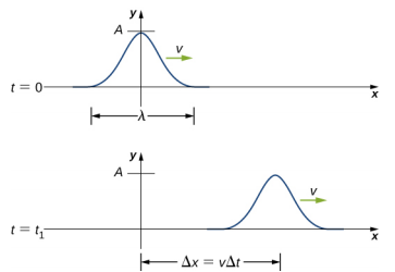
A pulse can be described as wave consisting of a single disturbance that moves through the medium with a constant amplitude. The pulse moves as a pattern that maintains its shape as it propagates with a constant wave speed. Because the wave speed is constant, the distance the pulse moves in a time Δt is equal to Δx = vΔt (Figure \(\PageIndex{1}\)).

Modeling a One-Dimensional Sinusoidal Wave Using a Wave Function
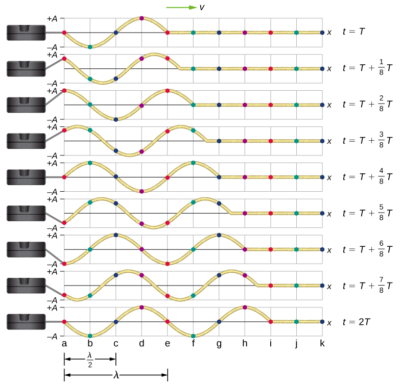
Consider a string kept at a constant tension \(F_T\) where one end is fixed and the free end is oscillated between \(y = +A\) and \(y = −A\) by a mechanical device at a constant frequency. Figure \(\PageIndex{2}\) shows snapshots of the wave at an interval of an eighth of a period, beginning after one period (\(t = T\)).

Notice that each select point on the string (marked by colored dots) oscillates up and down in simple harmonic motion, between \(y = +A\) and \(y = −A\), with a period \(T\). The wave on the string is sinusoidal and is translating in the positive x-direction as time progresses.
At this point, it is useful to recall from your study of algebra that if \(f(x)\) is some function, then \(f(x−d)\) is the same function translated in the positive x-direction by a distance \(d\). The function \(f(x+d)\) is the same function translated in the negative x-direction by a distance \(d\). We want to define a wave function that will give the \(y\)-position of each segment of the string for every position x along the string for every time \(t\).
Looking at the first snapshot in Figure \(\PageIndex{2}\), the y-position of the string between \(x = 0\) and \(x = λ\) can be modeled as a sine function. This wave propagates down the string one wavelength in one period, as seen in the last snapshot. The wave therefore moves with a constant wave speed of \(v = λ/T\).
Recall that a sine function is a function of the angle \(θ\), oscillating between +1 and −1, and repeating every \(2π\) radians (Figure \(\PageIndex{3}\)). However, the y-position of the medium, or the wave function, oscillates between \(+A\) and \(−A\), and repeats every wavelength \(λ\).

To construct our model of the wave using a periodic function, consider the ratio of the angle and the position,
\[\begin{align*} \dfrac{\theta}{x} &=\frac{2 \pi}{\lambda}, \\[4pt] \theta &=\frac{2 \pi}{\lambda} x. \end{align*}\]
Using \(\theta = \frac{2\pi}{\lambda}x\) and multiplying the sine function by the amplitude A, we can now model the y-position of the string as a function of the position x:
\[ y(x)=A \sin \left(\frac{2 \pi}{\lambda} x\right). \nonumber \]
The wave on the string travels in the positive x-direction with a constant velocity v, and moves a distance vt in a time t. The wave function can now be defined by
\[ y(x, t)=A \sin \left(\frac{2 \pi}{\lambda}(x-v t)\right). \nonumber \]
It is often convenient to rewrite this wave function in a more compact form. Multiplying through by the ratio \(\frac{2\pi}{\lambda}\) leads to the equation
\[ y(x, t)=A \sin \left(\frac{2 \pi}{\lambda} x-\frac{2 \pi}{\lambda} v t\right). \nonumber \]
The value \(\frac{2\pi}{\lambda}\) is defined as the wave number. The symbol for the wave number is k and has units of inverse meters, m−1:
\[ k \equiv \frac{2 \pi}{\lambda} \label{16.2} \]
Recall from Oscillations that the angular frequency is defined as \(\omega \equiv \frac{2\pi}{T}\). The second term of the wave function becomes
\[\frac{2 \pi}{\lambda} v t=\frac{2 \pi}{\lambda}\left(\frac{\lambda}{T}\right) t=\frac{2 \pi}{T} t=\omega t. \nonumber \]
The wave function for a simple harmonic wave on a string reduces to
\[ y(x, t)=A \sin (k x \mp \omega t) \nonumber \]
where A is the amplitude, \(k = \frac{2\pi}{\lambda}\) is the wave number, \(\omega = \frac{2\pi}{T}\) is the angular frequency, the minus sign is for waves moving in the positive x-direction, and the plus sign is for waves moving in the negative x-direction. The velocity of the wave is equal to
\[ v=\frac{\lambda}{T}=\frac{\lambda}{T}\left(\frac{2 \pi}{2 \pi}\right)=\frac{\omega}{k} \label{16.3} .\]
Think back to our discussion of a mass on a spring, when the position of the mass was modeled as
\[x(t) = A \cos(ωt+ϕ). \nonumber\]
The angle \(ϕ\) is a phase shift, added to allow for the fact that the mass may have initial conditions other than \(x = +A\) and \(v = 0\). For similar reasons, the initial phase is added to the wave function. The wave function modeling a sinusoidal wave, allowing for an initial phase shift \(ϕ\), is
\[ y(x, t)=A \sin (k x \mp \omega t+\phi) \label{16.4} \]
The value
\[ (k x \mp \omega t+\phi) \label{16.5} \]
is known as the phase of the wave, where \(\phi\) is the initial phase of the wave function. Whether the temporal term \(\omega t\) is negative or positive depends on the direction of the wave. First consider the minus sign for a wave with an initial phase equal to zero (\(\phi\) = 0). The phase of the wave would be (\(kx = \omega t\)). Consider following a point on a wave, such as a crest. A crest will occur when \(\sin(kx - \omega t = 1.00\), that is, when \(k x-\omega t=n \pi+\frac{\pi}{2}\), for any integral value of n. For instance, one particular crest occurs at \(k x-\omega t=\frac{\pi}{2}\). As the wave moves, time increases and x must also increase to keep the phase equal to \(\frac{\pi}{2}\). Therefore, the minus sign is for a wave moving in the positive x-direction. Using the plus sign, \(k x+\omega t=\frac{\pi}{2}\). As time increases, x must decrease to keep the phase equal to \(\frac{\pi}{2}\). The plus sign is used for waves moving in the negative x-direction. In summary, \(y(x, t)=A \sin (k x-\omega t+\phi)\) models a wave moving in the positive x-direction and \(y(x, t)=A \sin (k x+\omega t+\phi)\) models a wave moving in the negative x-direction.
Equation \ref{16.4} is known as a simple harmonic wave function. A wave function is any function such that \(f(x, t)=f(x-v t)\). Later in this chapter, we will see that it is a solution to the linear wave equation. Note that \(y(x, t)=A \cos \left(k x+\omega t+\phi^{\prime}\right)\) works equally well because it corresponds to a different phase shift \(\phi^{\prime}=\phi-\frac{\pi}{2}\).
- To find the amplitude, wavelength, period, and frequency of a sinusoidal wave, write down the wave function in the form \(y(x, t)=A \sin (k x-\omega t+\phi)\).
- The amplitude can be read straight from the equation and is equal to \(A\).
- The period of the wave can be derived from the angular frequency \( \left(T=\frac{2 \pi}{\omega}\right)\).
- The frequency can be found using \(f = \frac{1}{T}\)
- The wavelength can be found using the wave number \(\left(\lambda=\frac{2 \pi}{k}\right)\).
A transverse wave on a taut string is modeled with the wave function
\[ \begin{align*} y(x, t) &=A \sin (k x-w t) \\[4pt] &= (0.2 \: \mathrm{m}) \sin \left(6.28 \: \mathrm{m}^{-1} x-1.57 \: \mathrm{s}^{-1} t\right) \end{align*} \]
Find the amplitude, wavelength, period, and speed of the wave.
Strategy
All these characteristics of the wave can be found from the constants included in the equation or from simple combinations of these constants.
Solution
1. The amplitude, wave number, and angular frequency can be read directly from the wave equation:
\begin{align*}
y(x, t)=& A \sin (k x-w t)=0.2 \: \mathrm{m} \sin \left(6.28 \: \mathrm{m}^{-1} x-1.57 \: \mathrm{s}^{-1} t\right) \nonumber \\
&\left(A=0.2 \: \mathrm{m} ; k=6.28 \: \mathrm{m}^{-1} ; \omega=1.57 \: \mathrm{s}^{-1}\right) \nonumber
\end{align*}
2. The wave number can be used to find the wavelength:
\begin{array}{l}
k=\frac{2 \pi}{\lambda} \\
\lambda=\frac{2 \pi}{k}=\frac{2 \pi}{6.28 \: \mathrm{m}^{-1}}=1.0 \: \mathrm{m}
\end{array}
3. The period of the wave can be found using the angular frequency:
\begin{array}{l}
\omega=\frac{2 \pi}{T} \\
T=\frac{2 \pi}{\omega}=\frac{2 \pi}{1.57 \: \mathrm{s}^{-1}}=4 \: \mathrm{s}
\end{array}
4. The speed of the wave can be found using the wave number and the angular frequency. The direction of the wave can be determined by considering the sign of \(k x \mp \omega t\): A negative sign suggests that the wave is moving in the positive x-direction:
\[ |v|=\frac{\omega}{k}=\frac{1.57 \: \mathrm{s}^{-1}}{6.28 \: \mathrm{m}^{-1}}=0.25 \: \mathrm{m} / \mathrm{s} \nonumber\]
Significance
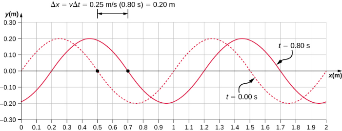
All of the characteristics of the wave are contained in the wave function. Note that the wave speed is the speed of the wave in the direction parallel to the motion of the wave. Plotting the height of the medium y versus the position x for two times t = 0.00 s and t = 0.80 s can provide a graphical visualization of the wave (Figure \(\PageIndex{4}\)).

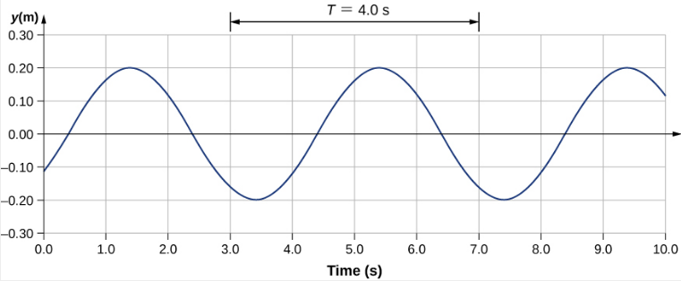
There is a second velocity to the motion. In this example, the wave is transverse, moving horizontally as the medium oscillates up and down perpendicular to the direction of motion. The graph in Figure \(\PageIndex{5}\) shows the motion of the medium at point x = 0.60 m as a function of time. Notice that the medium of the wave oscillates up and down between y = +0.20 m and y = −0.20 m every period of 4.0 seconds.

The wave function above is derived using a sine function. Can a cosine function be used instead?
Velocity and Acceleration of the Medium
As seen in Example \(\PageIndex{2}\), the wave speed is constant and represents the speed of the wave as it propagates through the medium, not the speed of the particles that make up the medium. The particles of the medium oscillate around an equilibrium position as the wave propagates through the medium. In the case of the transverse wave propagating in the x-direction, the particles oscillate up and down in the y-direction, perpendicular to the motion of the wave. The velocity of the particles of the medium is not constant, which means there is an acceleration. The velocity of the medium, which is perpendicular to the wave velocity in a transverse wave, can be found by taking the partial derivative of the position equation with respect to time. The partial derivative is found by taking the derivative of the function, treating all variables as constants, except for the variable in question. In the case of the partial derivative with respect to time \(t\), the position \(x\) is treated as a constant. Although this may sound strange if you haven’t seen it before, the object of this exercise is to find the transverse velocity at a point, so in this sense, the \(x\)-position is not changing. We have
\[\begin{split} y(x,t) & = A \sin (kx - \omega t + \phi) \\ v_{y} (x,t) & = \frac{\partial y(x,t)}{\partial t} = \frac{\partial}{\partial t} [A \sin (kx - \omega t + \phi)] \\ & = -A \omega \cos (kx - \omega t + \phi) \\ & = -v_{y\; max} \cos (kx - \omega t + \phi) \ldotp \end{split}\]
The magnitude of the maximum velocity of the medium is \(|v_{y\, max}| = A \omega\). This may look familiar from the Oscillations and a mass on a spring.
We can find the acceleration of the medium by taking the partial derivative of the velocity equation with respect to time,
\[\begin{split} a_{y} (x,t) & = \frac{\partial v_{y}(x,t)}{\partial t} = \frac{\partial}{\partial t} [-A \omega \cos (kx - \omega t + \phi)] \\ & = -A \omega^{2} \sin (kx - \omega t + \phi) \\ & = -a_{y\; max} \sin (kx - \omega t + \phi) \ldotp \end{split}\]
The magnitude of the maximum acceleration is |ay max| = A\(\omega^{2}\). The particles of the medium, or the mass elements, oscillate in simple harmonic motion for a mechanical wave.
The Linear Wave Equation
We have just determined the velocity of the medium at a position x by taking the partial derivative, with respect to time, of the position y. For a transverse wave, this velocity is perpendicular to the direction of propagation of the wave. We found the acceleration by taking the partial derivative, with respect to time, of the velocity, which is the second time derivative of the position:
\[a_{y} (x,t) = \frac{\partial^{2} y(x,t)}{\partial t^{2}} = \frac{\partial^{2}}{\partial t^{2}} [A \sin(kx - \omega t + \phi)] = -A \omega^{2} \sin (kx - \omega t + \phi) \ldotp\]
Now consider the partial derivatives with respect to the other variable, the position x, holding the time constant. The first derivative is the slope of the wave at a point x at a time t,
\[slope = \frac{\partial y(x,t)}{\partial x} = \frac{\partial}{\partial x} [A \sin (kx - \omega t + \phi)] = Ak \cos (kx - \omega t + \phi) \ldotp\]
The second partial derivative expresses how the slope of the wave changes with respect to position—in other words, the curvature of the wave, where
\[curvature = \frac{\partial^{2} y(x,t)}{\partial x^{2}} = \frac{\partial^{2}}{\partial x^{2}} [A \sin (kx - \omega t + \phi)] = -Ak^{2} \sin (kx - \omega t + \phi) \ldotp\]
The ratio of the acceleration and the curvature leads to a very important relationship in physics known as the linear wave equation. Taking the ratio and using the equation v = \(\frac{\omega}{k}\) yields the linear wave equation (also known simply as the wave equation or the equation of a vibrating string),
\[\begin{split} \frac{\frac{\partial^{2} y(x,t)}{\partial t^{2}}}{\frac{\partial^{2} y(x,t)}{\partial x^{2}}} & = \frac{-A \omega^{2} \sin (kx - \omega t + \phi)}{-Ak^{2} \sin (kx - \omega t + \phi)} \\ & = \frac{\omega^{2}}{k^{2}} = v^{2}, \end{split}\]
\[\frac{\partial^{2} y(x,t)}{\partial x^{2}} = \frac{1}{v^{2}} \frac{\partial^{2} y(x,t)}{\partial t^{2}} \ldotp \label{16.6}\]
Equation \ref{16.6} is the linear wave equation, which is one of the most important equations in physics and engineering. We derived it here for a transverse wave, but it is equally important when investigating longitudinal waves. This relationship was also derived using a sinusoidal wave, but it successfully describes any wave or pulse that has the form y(x, t) = f(x ∓ vt). These waves result due to a linear restoring force of the medium—thus, the name linear wave equation. Any wave function that satisfies this equation is a linear wave function.
An interesting aspect of the linear wave equation is that if two wave functions are individually solutions to the linear wave equation, then the sum of the two linear wave functions is also a solution to the wave equation. Consider two transverse waves that propagate along the x-axis, occupying the same medium. Assume that the individual waves can be modeled with the wave functions y1(x, t) = f(x ∓ vt) and y2(x, t) = g(x ∓ vt), which are solutions to the linear wave equations and are therefore linear wave functions. The sum of the wave functions is the wave function
\[y_{1} (x,t) + y_{2} (x,t) = f(x \mp vt) + g(x \mp vt) \ldotp\]
Consider the linear wave equation:
\[\begin{split} \frac{\partial^{2} (f + g)}{\partial x^{2}} & = \frac{1}{v^{2}} \frac{\partial^{2} (f + g)}{\partial t^{2}} \\ \frac{\partial^{2} f}{\partial x^{2}} + \frac{\partial^{2} g}{\partial x^{2}} & = \frac{1}{v^{2}} \left(\dfrac{\partial^{2} f}{\partial t^{2}} + \frac{\partial^{2} g}{\partial t^{2}}\right) \ldotp \end{split}\]
This has shown that if two linear wave functions are added algebraically, the resulting wave function is also linear. This wave function models the displacement of the medium of the resulting wave at each position along the x-axis. If two linear waves occupy the same medium, they are said to interfere. If these waves can be modeled with a linear wave function, these wave functions add to form the wave equation of the wave resulting from the interference of the individual waves. The displacement of the medium at every point of the resulting wave is the algebraic sum of the displacements due to the individual waves.
Taking this analysis a step further, if wave functions y1 (x, t) = f(x ∓ vt) and y2 (x, t) = g(x ∓ vt) are solutions to the linear wave equation, then Ay1(x, t) + By2(x, y), where A and B are constants, is also a solution to the linear wave equation. This property is known as the principle of superposition. Interference and superposition are covered in more detail in Interference of Waves.
Consider a very long string held taut by two students, one on each end. Student A oscillates the end of the string producing a wave modeled with the wave function y1(x, t) = A sin(kx − \(\omega\)t) and student B oscillates the string producing at twice the frequency, moving in the opposite direction. Both waves move at the same speed v = \(\frac{\omega}{k}\). The two waves interfere to form a resulting wave whose wave function is yR(x, t) = y1(x, t) + y2(x, t). Find the velocity of the resulting wave using the linear wave equation \(\frac{\partial^{2} y(x,t)}{\partial x^{2}} = \frac{1}{v^{2}} \frac{\partial^{2} y(x,t)}{\partial t^{2}}\).
Strategy
First, write the wave function for the wave created by the second student. Note that the angular frequency of the second wave is twice the frequency of the first wave (2\(\omega\)), and since the velocity of the two waves are the same, the wave number of the second wave is twice that of the first wave (2k). Next, write the wave equation for the resulting wave function, which is the sum of the two individual wave functions. Then find the second partial derivative with respect to position and the second partial derivative with respect to time. Use the linear wave equation to find the velocity of the resulting wave.
Solution
- Write the wave function of the second wave: y2(x, t) = A sin(2kx + 2\(\omega\)t).
- Write the resulting wave function: $y_{R} (x,t) = y_{1} (x,t) + y(x,t) = A \sin (kx - \omega t) + A \sin (2kx + 2 \omega t) \ldotp$
- Find the partial derivatives: $\begin{split} \frac{\partial y_{R} (x,t)}{\partial x} & = -Ak \cos (kx - \omega t) + 2Ak \cos (2kx + 2 \omega t), \\ \frac{\partial^{2} y_{R} (x,t)}{\partial x^{2}} & = -Ak^{2} \sin (kx - \omega t) - 4Ak^{2} \sin(2kx + 2 \omega t), \\ \frac{\partial y_{R} (x,t)}{\partial t} & = -A \omega \cos (kx - \omega t) + 2A \omega \cos (2kx + 2 \omega t), \\ \frac{\partial^{2} y_{R} (x,t)}{\partial t^{2}} & = -A \omega^{2} \sin (kx - \omega t) - 4A \omega^{2} \sin(2kx + 2 \omega t) \ldotp \end{split}$
- Use the wave equation to find the velocity of the resulting wave: $\begin{split} \frac{\partial^{2} y(x,t)}{\partial x^{2}} & = \frac{1}{v^{2}} \frac{\partial^{2} y(x,t)}{\partial t^{2}}, \\ -Ak^{2} \sin (kx - \omega t) + 4Ak^{2} \sin(2kx + 2 \omega t) & = \frac{1}{v^{2}} \left(-A \omega^{2} \sin (kx - \omega t) - 4A \omega^{2} \sin(2kx + 2 \omega t)\right), \\ k^{2} \left(-A \sin (kx - \omega t) + 4A \sin(2kx + 2 \omega t)\right) & = \frac{\omega^{2}}{v^{2}} \left(-A \sin (kx - \omega t) - 4A \sin(2kx + 2 \omega t)\right), \\ k^{2} & = \frac{\omega^{2}}{v^{2}}, \\ |v| & = \frac{\omega}{k} \ldotp \end{split}$
Significance
The speed of the resulting wave is equal to the speed of the original waves \(\left(v = \frac{\omega}{k}\right)\). We will show in the next section that the speed of a simple harmonic wave on a string depends on the tension in the string and the mass per length of the string. For this reason, it is not surprising that the component waves as well as the resultant wave all travel at the same speed.
The wave equation \(\frac{\partial^{2} y(x,t)}{\partial x^{2}} = \frac{1}{v^{2}} \frac{\partial^{2} y(x,t)}{\partial t^{2}}\) works for any wave of the form y(x, t) = f(x ∓ vt). In the previous section, we stated that a cosine function could also be used to model a simple harmonic mechanical wave. Check if the wave
\[y(x,t) = (0.50\; m) \cos (0.20 \pi\; m^{-1} x - 4.00 \pi s^{-1} t + \frac{\pi}{10})\]
is a solution to the wave equation.
Any disturbance that complies with the wave equation can propagate as a wave moving along the x-axis with a wave speed v. It works equally well for waves on a string, sound waves, and electromagnetic waves. This equation is extremely useful. For example, it can be used to show that electromagnetic waves move at the speed of light.


