3.1: Position Vectors and Components

Vectors

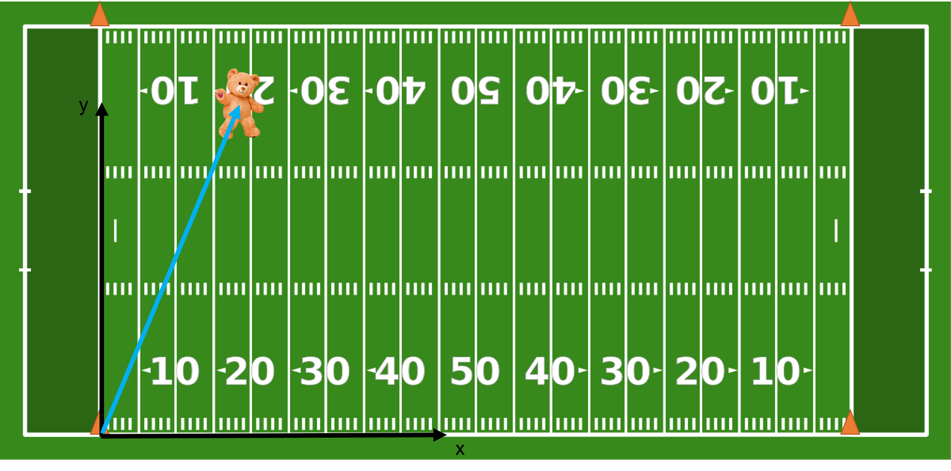
As we saw at the beginning of the chapter, vectors are a simple way of representing a value that has both a magnitude and a direction. One of the simplest things we can represent using vectors is the position of an object. Imagine you have a teddy bear somewhere on a football field.

Now, imagine you have forgotten it and you need to tell someone where to find it in the middle of the night.

First, you have to set up a coordinate system. This means you need to tell someone what direction your "x" values will go and what direction your "y" values will go. What we can do is say that going the length of the field will be our "x" direction and going across the field will be our "y" direction. We also need to say where we are going to be measuring from, in other words where do we start from. This is called our origin. We will set this in the bottom left corner at the orange cone. When we have done all of this, we will have the following.

Now that we have this all set up, we can draw a vector that points directly to the teddy bear!

Great, but this is getting pretty hard to see. Let's remove all of the distracting parts and just show the representations of everything:

where I've labeled the point the teddy bear is at "B" for Bear! The vector I will call \(r_B\). (For some reason, we often use the letter "r" for vectors that point to positions.

Great! Now we can see everything and start do do some math! First, the best way of representing a vector is by its components. You can think of components as telling someone how much to move in each direction to get to the bear. For instance, you may say that they should move 17 yards in the x-direction and 35 yards in the y-direction. (Apologies for using silly units like "yards" instead of nice units like "meters". That's American football for you! I promise not to do it again.) These measurements are called the x-component and y-component, respectively. You would say that \(r_B,x=17 \textrm{ yards}\) and \(r_B,y= 35 \textrm{ yards}\). We can show these components on the graph.

However, this will get cumbersome very quickly and I hate the double subscripts (although they are necessary sometimes). This representation will also be a real pain when we need to start adding and subtracting vectors. So, we will introduce a new represenation of vectors called column vector notation. Here is that same vector, \(r_B\) represented in column vector form:

\[ \vec{r_B}=\begin{bmatrix} r_B,x \\ r_B,y \end{bmatrix} =\begin{bmatrix} 17 \textrm{ yards} \\ 35 \textrm{ yards} \end{bmatrix} \label{2.10} \]

This is all looking great. But, what if the person getting your teddy bear is not starting at the origin? What do we do then?

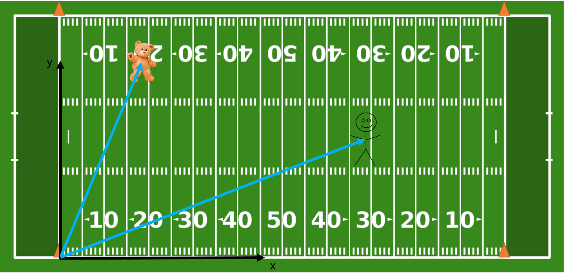
Well, of course now we need to construct our second position vector. To tell the person where to go, we also need a third vector. This will be called a displacement vector. This is just a vector that points from one point to another. However, unlike our position vectors, a displacement vector can start anywhere. We'll have our start at the person and point to the teddy bear.

As you can see, \(\Delta \vec{r}\) is the vector that points between point P and point B. This is where the person, P, would need to walk to get to the bear, B. How do we find this mathematically? Well, first we need to know the coordinates of point P. Let's say \(\vec{r_P}=\begin{bmatrix} 68 \textrm{ yards} \\ 16 \textrm{ yards} \end{bmatrix}\). Now, to get the displacement vector, \(\Delta \vec{r}\), we simply subtract the components of vector \(r_P\) from the components of \(r_B\).

\[ \Delta \vec{r}=\begin{bmatrix} r_B,x \\ r_B,y \end{bmatrix} - \begin{bmatrix} r_P,x \\ r_P,y \end{bmatrix} \label{2.11} \]

\[ \Delta \vec{r}=\begin{bmatrix} 17 \textrm{ yards} \\ 35 \textrm{ yards} \end{bmatrix} - \begin{bmatrix} 68 \textrm{ yards} \\ 16 \textrm{ yards} \end{bmatrix} \label{2.12} \]

\[ \Delta \vec{r}=\begin{bmatrix} -51 \textrm{ yards} \\ 19 \textrm{ yards} \end{bmatrix} \label{2.13} \]

So, this is the vector that says where the person should walk to get to the teddy bare from where they are currently standing.

We may want to express this vector in different ways. If we want to know how far the person needs to walk, we just use the Pythagorean theorem. This is just the magnitude of the vector. We normally indicate this with an absolute value sign around the vector, \( | \Delta \vec{r}|\).

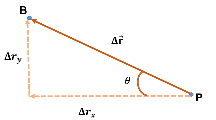\[ |\Delta \vec{r}|=\sqrt{\Delta r_x^2 + \Delta r_y^2}= \sqrt{(-51\textrm{ yards})^2+(19\textrm{ yards})^2} = 54.4 \textrm{ yards} \label{2.14} \]

And we can find the angle by using \(\sin\), \(\cos\), or \(\tan\) functions. I will use \(\tan\), as it does not rely on me getting the magnitude of \(|\Delta \vec{r}|\) correct.

\[ \theta = \tan \frac{\Delta r_y}{\Delta r_x} = \tan \frac{19}{51} = 20.4^{\circ} \label{2.15} \]

So now, we can just tell our helper to walk 54.4 yards at an angle \(20.4^{\circ}\) above the x-axis.

Vectors in 3 Dimensions

The last thing we should do is extend this into three dimensions. After all, we live in a (spatially) 3D world. The good news is that this is easy! Just add one more component (the z-component) to your column vector! For a 3-dimensional column vector, \(\vec(A)\), we will have:

\[ \vec{A}=\begin{bmatrix} A_x \\ A_y \\ A_Z \end{bmatrix} \label{2.16} \]

This is pretty straightforward. Luckily, it is rare that we encounter a 3-dimensional problem, so often you will be setting one of these components to zero.

In the next section, we will learn how to do math with vectors in one dimension and the two dimensions.