
2.11.2: Voltage Related To Field


- Last updated
- Mar 8, 2021
- Save as PDF

( \newcommand{\kernel}{\mathrm{null}\,}\)
10.2.1 One dimension
Voltage is electrical energy per unit charge, and electric field is force per unit charge. For a particle moving in one dimension, along the x axis, we can therefore relate voltage and field if we start from the relationship between interaction energy and force,
and divide by charge,
giving
or
The interpretation is that a strong electric field occurs in a region of space where the voltage is rapidly changing. By analogy, a steep hillside is a place on the map where the altitude is rapidly changing.
| Example 6: Field generated by an electric eel |
|---|
| ▹ Suppose an electric eel is 1 m long, and generates a voltage difference of 1000 volts between its head and tail. What is the electric field in the water around it? ▹ We are only calculating the amount of field, not its direction, so we ignore positive and negative signs. Subject to the possibly inaccurate assumption of a constant field parallel to the eel's body, we have |E|=dVdx≈ΔVΔx[assumption of constant field]=1000 V/m. |
| Example 7: Relating the units of electric field and voltage |
|---|
| From our original definition of the electric field, we expect it to have units of newtons per coulomb, N/C. The example above, however, came out in volts per meter, V/m. Are these inconsistent? Let's reassure ourselves that this all works. In this kind of situation, the best strategy is usually to simplify the more complex units so that they involve only mks units and coulombs. Since voltage is defined as electrical energy per unit charge, it has units of J/C: Vm=J/Cm=JC⋅m. To connect joules to newtons, we recall that work equals force times distance, so J=N⋅m, so Vm=N⋅mC⋅m=NC As with other such difficulties with electrical units, one quickly begins to recognize frequently occurring combinations. |
| Example 8: Voltage associated with a point charge |
|---|
| ▹ What is the voltage associated with a point charge? ▹ As derived previously in self-check A on page 563, the field is |E|=kQr2 The difference in voltage between two points on the same radius line is ΔV=−∫dV=−∫Exdx In the general discussion above, x was just a generic name for distance traveled along the line from one point to the other, so in this case x really means r. ΔV=−∫r2r1Erdr=−∫r2r1kQr2dr=kQr]r2r1 =kQr2−kQr1. The standard convention is to use r1=∞ as a reference point, so that the voltage at any distance r from the charge is V=kQr. The interpretation is that if you bring a positive test charge closer to a positive charge, its electrical energy is increased; if it was released, it would spring away, releasing this as kinetic energy. |
self-check:
Show that you can recover the expression for the field of a point charge by evaluating the derivative Ex=−dV/dx.
(answer in the back of the PDF version of the book)
10.2.2 Two or three dimensions
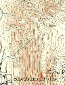
a / A topographical map of Shelburne Falls, Mass. (USGS).
The topographical map in figure a suggests a good way to visualize the relationship between field and voltage in two dimensions. Each contour on the map is a line of constant height; some of these are labeled with their elevations in units of feet. Height is related to gravitational energy, so in a gravitational analogy, we can think of height as representing voltage. Where the contour lines are far apart, as in the town, the slope is gentle. Lines close together indicate a steep slope.
If we walk along a straight line, say straight east from the town, then height (voltage) is a function of the east-west coordinate x. Using the usual mathematical definition of the slope, and writing V for the height in order to remind us of the electrical analogy, the slope along such a line is dV/dx (the rise over the run).
What if everything isn't confined to a straight line? Water flows downhill. Notice how the streams on the map cut perpendicularly through the lines of constant height.
It is possible to map voltages in the same way, as shown in figure b. The electric field is strongest where the constant-voltage curves are closest together, and the electric field vectors always point perpendicular to the constant-voltage curves.
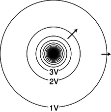
b / The constant-voltage curves surrounding a point charge. Near the charge, the curves are so closely spaced that they blend together on this drawing due to the finite width with which they were drawn. Some electric fields are shown as arrows.
The one-dimensional relationship E=−dV/dx generalizes to three dimensions as follows:
This can be notated as a gradient (page 215),
and if we know the field and want to find the voltage, we can use a line integral,
where the quantity inside the integral is a vector dot product.
self-check:
Imagine that figure a represents voltage rather than height. (a) Consider the stream the starts near the center of the map. Determine the positive and negative signs of dV/dx and dV/dy, and relate these to the direction of the force that is pushing the current forward against the resistance of friction. (b) If you wanted to find a lot of electric charge on this map, where would you look?
(answer in the back of the PDF version of the book)
Figure c shows some examples of ways to visualize field and voltage patterns.
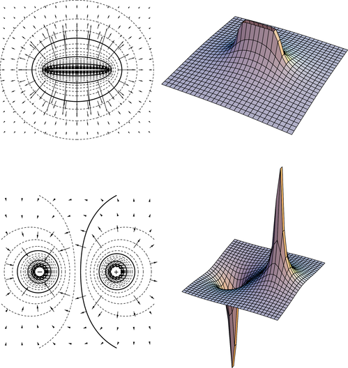
c / Two-dimensional field and voltage patterns. Top: A uniformly charged rod. Bottom: A dipole. In each case, the diagram on the left shows the field vectors and constant-voltage curves, while the one on the right shows the voltage (up-down coordinate) as a function of x and y. Interpreting the field diagrams: Each arrow represents the field at the point where its tail has been positioned. For clarity, some of the arrows in regions of very strong field strength are not shown --- they would be too long to show. Interpreting the constant-voltage curves: In regions of very strong fields, the curves are not shown because they would merge together to make solid black regions. Interpreting the perspective plots: Keep in mind that even though we're visualizing things in three dimensions, these are really two-dimensional voltage patterns being represented. The third (up-down) dimension represents voltage, not position.
Contributors
Benjamin Crowell (Fullerton College). Conceptual Physics is copyrighted with a CC-BY-SA license.