2.2: Speed and Velocity
- Last updated
- Jun 17, 2019
- Save as PDF
- Page ID
- 17858

- Boundless
- Boundless
( \newcommand{\kernel}{\mathrm{null}\,}\)
Average Velocity: A Graphical Interpretation
Average velocity is defined as the change in position (or displacement) over the time of travel.
learning objectives
- Contrast speed and velocity in physics
In everyday usage, the terms “speed” and “velocity” are used interchangeably. In physics, however, they are distinct quantities. Speed is a scalar quantity and has only magnitude. Velocity, on the other hand, is a vector quantity and so has both magnitude and direction. This distinction becomes more apparent when we calculate average speed and velocity.
Average speed is calculated as the distance traveled over the total time of travel. In contrast, average velocity is defined as the change in position (or displacement) over the total time of travel.

Average Velocity: The kinematic formula for calculating average velocity is the change in position over the time of travel.
The SI unit for velocity is meters per second, or m/s, but many other units (such as km/h, mph, and cm/s) are commonly used. Suppose, for example, an airplane passenger took five seconds to move -4 m (the negative sign indicates that displacement is toward the back of the plane ). His average velocity would be:
v=Δxt=−4m5s=−0.8ms
The minus sign indicates that the average velocity is also toward the rear of the plane.
The average velocity of an object does not tell us anything about what happens to it between the starting point and ending point, however. For example, we cannot tell from average velocity whether the airplane passenger stops momentarily or backs up before he gets to the back of the plane. To get more details, we must consider smaller segments of the trip over smaller time intervals.
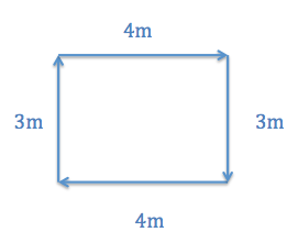
To illustrate the difference between average speed and average velocity, consider the following additional example. Imagine you are walking in a small rectangle. You walk three meters north, four meters east, three meters south, and another four meters west. The entire walk takes you 30 seconds. If you are calculating average speed, you would calculate the entire distance (3 + 4 + 3 + 4 = 14 meters) over the total time, 30 seconds. From this, you would get an average speed of 14/30 = 0.47 m/s. When calculating average velocity, however, you are looking at the displacement over time. Because you walked in a full rectangle and ended up exactly where you started, your displacement is 0 meters. Therefore, your average velocity, or displacement over time, would be 0 m/s.

Average Speed vs. Average Velocity: If you started walking from one corner and went all the way around the rectangle in 30 seconds, your average speed would be 0.47 m/s, but your average velocity would be 0 m/s.
Instananeous Velocity: A Graphical Interpretation
Instantaneous velocity is the velocity of an object at a single point in time and space as calculated by the slope of the tangent line.
learning objectives
- Differentiate instantaneous velocity from other ways of determining velocity
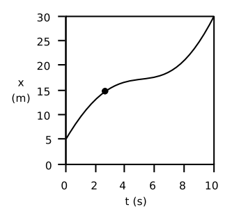
Typically, motion is not with constant velocity nor speed. While driving in a car, for example, we continuously speed up and slow down. A graphical representation of our motion in terms of distance vs. time, therefore, would be more variable or “curvy” rather than a straight line, indicating motion with a constant velocity as shown below. (We limit our discussion to one dimensional motion. It should be straightforward to generalize to three dimensional cases.)

Motion with Changing Velocity: Motion is often observed with changing velocity. This would result in a curvy line when graphed with distance over time.
To calculate the speed of an object from a graph representing constant velocity, all that is needed is to find the slope of the line; this would indicate the change in distance over the change in time. However, changing velocity it is not as straightforward.
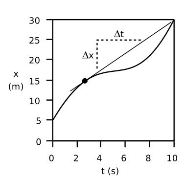
Since our velocity is constantly changing, we can estimate velocity in different ways. One way is to look at our instantaneous velocity, represented by one point on our curvy line of motion graphed with distance vs. time. In order to determine our velocity at any given moment, we must determine the slope at that point. To do this, we find a line that represents our velocity in that moment, shown graphically in. That line would be the line tangent to the curve at that point. If we extend this line, we can easily calculate the displacement of distance over time and determine our velocity at that given point. The velocity of an object at any given moment is the slope of the tangent line through the relevant point on its x vs. t graph.

Determining instantaneous velocity: The velocity at any given moment is defined as the slope of the tangent line through the relevant point on the graph
Instantaneous Velocity, Acceleration, Jerk, Slopes, Graphs vs. Time: This is how kinematics begins.
In calculus, finding the slope of curve f(x) at x=x0x=x0 is equivalent to finding the first derivative:
df(x)dx|x=x0.
One interpretation of this definition is that the velocity shows how many meters the object would travel in one second if it continues moving at the same speed for at least one second.
Key Points
- Average velocity can be calculated by determining the total displacement divided by the total time of travel.
- The average velocity of an object does not tell us anything about what happens to it between the starting point and ending point.
- Average velocity is different from average speed in that it considers the direction of travel and the overall change in position.
- When velocity is constantly changing, we can estimate our velocity by looking at instantaneous velocity.
- Instantaneous velocity is calculated by determining the slope of the line tangent to the curve at the point of interest.
- Instantaneous velocity is similar to determining how many meters the object would travel in one second at a specific moment.
Key Terms
- velocity: A vector quantity that denotes the rate of change of position with respect to time, or a speed with a directional component.
- instantaneous: (As in velocity)—occurring, arising, or functioning without any delay; happening within an imperceptibly brief period of time.
LICENSES AND ATTRIBUTIONS
CC LICENSED CONTENT, SHARED PREVIOUSLY
- Curation and Revision. Provided by: Boundless.com. License: CC BY-SA: Attribution-ShareAlike
CC LICENSED CONTENT, SPECIFIC ATTRIBUTION
- OpenStax College, College Physics. September 17, 2013. Provided by: OpenStax CNX. Located at: http://cnx.org/content/m42096/latest/?collection=col11406/1.7. License: CC BY: Attribution
- velocity. Provided by: Wiktionary. Located at: en.wiktionary.org/wiki/velocity. License: CC BY-SA: Attribution-ShareAlike
- OpenStax College, College Physics. October 20, 2012. Provided by: OpenStax CNX. Located at: http://cnx.org/content/m42096/latest/?collection=col11406/1.7. License: CC BY: Attribution
- Provided by: None. Located at: None. License: CC BY-SA: Attribution-ShareAlike
- Provided by: Light and Matter. Located at: http://lightandmatter.com/lmb.pdf. License: CC BY: Attribution
- instantaneous. Provided by: Wiktionary. Located at: en.wiktionary.org/wiki/instantaneous. License: CC BY-SA: Attribution-ShareAlike
- OpenStax College, College Physics. October 20, 2012. Provided by: OpenStax CNX. Located at: http://cnx.org/content/m42096/latest/?collection=col11406/1.7. License: CC BY: Attribution
- Provided by: None. Located at: None. License: CC BY-SA: Attribution-ShareAlike
- Provided by: Light and Matter. Located at: http://lightandmatter.com/lmb.pdf. License: CC BY: Attribution
- Instantaneous Velocity, Acceleration, Jerk, Slopes, Graphs vs. Time. Located at: http://www.youtube.com/watch?v=STcgrV2L4tw. License: Public Domain: No Known Copyright. License Terms: Standard YouTube license
- Provided by: Light and Matter. Located at: http://lightandmatter.com/lmb.pdf. License: CC BY: Attribution


