Physics LibreTexts

11.14: Angular Acceleration

  • Page ID
    18261
    • Boundless
    • Boundless

    \( \newcommand{\vecs}[1]{\overset { \scriptstyle \rightharpoonup} {\mathbf{#1}} } \)

    \( \newcommand{\vecd}[1]{\overset{-\!-\!\rightharpoonup}{\vphantom{a}\smash {#1}}} \)

    \( \newcommand{\id}{\mathrm{id}}\) \( \newcommand{\Span}{\mathrm{span}}\)

    ( \newcommand{\kernel}{\mathrm{null}\,}\) \( \newcommand{\range}{\mathrm{range}\,}\)

    \( \newcommand{\RealPart}{\mathrm{Re}}\) \( \newcommand{\ImaginaryPart}{\mathrm{Im}}\)

    \( \newcommand{\Argument}{\mathrm{Arg}}\) \( \newcommand{\norm}[1]{\| #1 \|}\)

    \( \newcommand{\inner}[2]{\langle #1, #2 \rangle}\)

    \( \newcommand{\Span}{\mathrm{span}}\)

    \( \newcommand{\id}{\mathrm{id}}\)

    \( \newcommand{\Span}{\mathrm{span}}\)

    \( \newcommand{\kernel}{\mathrm{null}\,}\)

    \( \newcommand{\range}{\mathrm{range}\,}\)

    \( \newcommand{\RealPart}{\mathrm{Re}}\)

    \( \newcommand{\ImaginaryPart}{\mathrm{Im}}\)

    \( \newcommand{\Argument}{\mathrm{Arg}}\)

    \( \newcommand{\norm}[1]{\| #1 \|}\)

    \( \newcommand{\inner}[2]{\langle #1, #2 \rangle}\)

    \( \newcommand{\Span}{\mathrm{span}}\) \( \newcommand{\AA}{\unicode[.8,0]{x212B}}\)

    \( \newcommand{\vectorA}[1]{\vec{#1}}      % arrow\)

    \( \newcommand{\vectorAt}[1]{\vec{\text{#1}}}      % arrow\)

    \( \newcommand{\vectorB}[1]{\overset { \scriptstyle \rightharpoonup} {\mathbf{#1}} } \)

    \( \newcommand{\vectorC}[1]{\textbf{#1}} \)

    \( \newcommand{\vectorD}[1]{\overrightarrow{#1}} \)

    \( \newcommand{\vectorDt}[1]{\overrightarrow{\text{#1}}} \)

    \( \newcommand{\vectE}[1]{\overset{-\!-\!\rightharpoonup}{\vphantom{a}\smash{\mathbf {#1}}}} \)

    \( \newcommand{\vecs}[1]{\overset { \scriptstyle \rightharpoonup} {\mathbf{#1}} } \)

    \( \newcommand{\vecd}[1]{\overset{-\!-\!\rightharpoonup}{\vphantom{a}\smash {#1}}} \)

    \(\newcommand{\avec}{\mathbf a}\) \(\newcommand{\bvec}{\mathbf b}\) \(\newcommand{\cvec}{\mathbf c}\) \(\newcommand{\dvec}{\mathbf d}\) \(\newcommand{\dtil}{\widetilde{\mathbf d}}\) \(\newcommand{\evec}{\mathbf e}\) \(\newcommand{\fvec}{\mathbf f}\) \(\newcommand{\nvec}{\mathbf n}\) \(\newcommand{\pvec}{\mathbf p}\) \(\newcommand{\qvec}{\mathbf q}\) \(\newcommand{\svec}{\mathbf s}\) \(\newcommand{\tvec}{\mathbf t}\) \(\newcommand{\uvec}{\mathbf u}\) \(\newcommand{\vvec}{\mathbf v}\) \(\newcommand{\wvec}{\mathbf w}\) \(\newcommand{\xvec}{\mathbf x}\) \(\newcommand{\yvec}{\mathbf y}\) \(\newcommand{\zvec}{\mathbf z}\) \(\newcommand{\rvec}{\mathbf r}\) \(\newcommand{\mvec}{\mathbf m}\) \(\newcommand{\zerovec}{\mathbf 0}\) \(\newcommand{\onevec}{\mathbf 1}\) \(\newcommand{\real}{\mathbb R}\) \(\newcommand{\twovec}[2]{\left[\begin{array}{r}#1 \\ #2 \end{array}\right]}\) \(\newcommand{\ctwovec}[2]{\left[\begin{array}{c}#1 \\ #2 \end{array}\right]}\) \(\newcommand{\threevec}[3]{\left[\begin{array}{r}#1 \\ #2 \\ #3 \end{array}\right]}\) \(\newcommand{\cthreevec}[3]{\left[\begin{array}{c}#1 \\ #2 \\ #3 \end{array}\right]}\) \(\newcommand{\fourvec}[4]{\left[\begin{array}{r}#1 \\ #2 \\ #3 \\ #4 \end{array}\right]}\) \(\newcommand{\cfourvec}[4]{\left[\begin{array}{c}#1 \\ #2 \\ #3 \\ #4 \end{array}\right]}\) \(\newcommand{\fivevec}[5]{\left[\begin{array}{r}#1 \\ #2 \\ #3 \\ #4 \\ #5 \\ \end{array}\right]}\) \(\newcommand{\cfivevec}[5]{\left[\begin{array}{c}#1 \\ #2 \\ #3 \\ #4 \\ #5 \\ \end{array}\right]}\) \(\newcommand{\mattwo}[4]{\left[\begin{array}{rr}#1 \amp #2 \\ #3 \amp #4 \\ \end{array}\right]}\) \(\newcommand{\laspan}[1]{\text{Span}\{#1\}}\) \(\newcommand{\bcal}{\cal B}\) \(\newcommand{\ccal}{\cal C}\) \(\newcommand{\scal}{\cal S}\) \(\newcommand{\wcal}{\cal W}\) \(\newcommand{\ecal}{\cal E}\) \(\newcommand{\coords}[2]{\left\{#1\right\}_{#2}}\) \(\newcommand{\gray}[1]{\color{gray}{#1}}\) \(\newcommand{\lgray}[1]{\color{lightgray}{#1}}\) \(\newcommand{\rank}{\operatorname{rank}}\) \(\newcommand{\row}{\text{Row}}\) \(\newcommand{\col}{\text{Col}}\) \(\renewcommand{\row}{\text{Row}}\) \(\newcommand{\nul}{\text{Nul}}\) \(\newcommand{\var}{\text{Var}}\) \(\newcommand{\corr}{\text{corr}}\) \(\newcommand{\len}[1]{\left|#1\right|}\) \(\newcommand{\bbar}{\overline{\bvec}}\) \(\newcommand{\bhat}{\widehat{\bvec}}\) \(\newcommand{\bperp}{\bvec^\perp}\) \(\newcommand{\xhat}{\widehat{\xvec}}\) \(\newcommand{\vhat}{\widehat{\vvec}}\) \(\newcommand{\uhat}{\widehat{\uvec}}\) \(\newcommand{\what}{\widehat{\wvec}}\) \(\newcommand{\Sighat}{\widehat{\Sigma}}\) \(\newcommand{\lt}{<}\) \(\newcommand{\gt}{>}\) \(\newcommand{\amp}{&}\) \(\definecolor{fillinmathshade}{gray}{0.9}\)

    learning objectives

    • Relate angle of rotation, angular velocity, and angular acceleration to their equivalents in linear kinematics

    Simply by using our intuition, we can begin to see the interrelatedness of rotational quantities like θ (angle of rotation), ω(angular velocity) and α (angular acceleration). For example, if a motorcycle wheel has a large angular acceleration for a fairly long time, it ends up spinning rapidly and rotating through many revolutions. The wheel’s rotational motion is analogous to the fact that the motorcycle’s large translational acceleration produces a large final velocity, and the distance traveled will also be large.

    Kinematic Equations

    Kinematics is the description of motion. We have already studied kinematic equations governing linear motion under constant acceleration:

    \[\begin{align} \mathrm{v} & \mathrm{=v_0+at} \\ \mathrm{x} & \mathrm{=v_0t+\frac{1}{2}at^2} \\ \mathrm{v^2} & \mathrm{=v_0^2+2ax} \end{align}\]

    Similarly, the kinematics of rotational motion describes the relationships among rotation angle, angular velocity, angular acceleration, and time. Let us start by finding an equation relating ω, α, and t. To determine this equation, we use the corresponding equation for linear motion:

    \[\mathrm{v=v_0+at.}\]

    As in linear kinematics where we assumed a is constant, here we assume that angular acceleration α is a constant, and can use the relation: \(\mathrm{a=rα}\) Where r – radius of curve.Similarly, we have the following relationships between linear and angular values:

    \[\begin{align} \mathrm{v} & \mathrm{=rω} \\ \mathrm{x} & \mathrm{=rθ} \end{align}\]

    By using the relationships \(\mathrm{a=rα, v=rω,}\) and \(\mathrm{x=rθ}\), we derive all the other kinematic equations for rotational motion under constant acceleration:

    \[\begin{align} \mathrm{ω} & \mathrm{=ω_0+αt} \\ \mathrm{θ} & \mathrm{=ω_0t+\frac{1}{2}αt^2} \\ \mathrm{ω^2} & \mathrm{= ω_0^2+2αθ} \end{align}\]

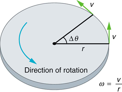
    The equations given above can be used to solve any rotational or translational kinematics problem in which a and α are constant. shows the relationship between some of the quantities discussed in this atom.
    image

    Linear and Angular: This figure shows uniform circular motion and some of its defined quantities.

    Key Points

    • The kinematic equations for rotational and/or linear motion given here can be used to solve any rotational or translational kinematics problem in which a and α are constant.
    • By using the relationships between velocity and angular velocity, distance and angle of rotation, and acceleration and angular acceleration, rotational kinematic equations can be derived from their linear motion counterparts.
    • To derive rotational equations from the linear counterparts, we used the relationships \(\mathrm{a=rα, v=rω,}\) and \(\mathrm{x=rθ}\).

    Key Terms

    • kinematics: The branch of mechanics concerned with objects in motion, but not with the forces involved.
    • angular: Relating to an angle or angles; having an angle or angles; forming an angle or corner; sharp-cornered; pointed; as in, an angular figure.

    LICENSES AND ATTRIBUTIONS

    CC LICENSED CONTENT, SHARED PREVIOUSLY

    CC LICENSED CONTENT, SPECIFIC ATTRIBUTION


    This page titled 11.14: Angular Acceleration is shared under a not declared license and was authored, remixed, and/or curated by Boundless.

    • Was this article helpful?