Physics LibreTexts

9.1: Introduction

  • Page ID
    100420
  • \( \newcommand{\vecs}[1]{\overset { \scriptstyle \rightharpoonup} {\mathbf{#1}} } \)

    \( \newcommand{\vecd}[1]{\overset{-\!-\!\rightharpoonup}{\vphantom{a}\smash {#1}}} \)

    \( \newcommand{\id}{\mathrm{id}}\) \( \newcommand{\Span}{\mathrm{span}}\)

    ( \newcommand{\kernel}{\mathrm{null}\,}\) \( \newcommand{\range}{\mathrm{range}\,}\)

    \( \newcommand{\RealPart}{\mathrm{Re}}\) \( \newcommand{\ImaginaryPart}{\mathrm{Im}}\)

    \( \newcommand{\Argument}{\mathrm{Arg}}\) \( \newcommand{\norm}[1]{\| #1 \|}\)

    \( \newcommand{\inner}[2]{\langle #1, #2 \rangle}\)

    \( \newcommand{\Span}{\mathrm{span}}\)

    \( \newcommand{\id}{\mathrm{id}}\)

    \( \newcommand{\Span}{\mathrm{span}}\)

    \( \newcommand{\kernel}{\mathrm{null}\,}\)

    \( \newcommand{\range}{\mathrm{range}\,}\)

    \( \newcommand{\RealPart}{\mathrm{Re}}\)

    \( \newcommand{\ImaginaryPart}{\mathrm{Im}}\)

    \( \newcommand{\Argument}{\mathrm{Arg}}\)

    \( \newcommand{\norm}[1]{\| #1 \|}\)

    \( \newcommand{\inner}[2]{\langle #1, #2 \rangle}\)

    \( \newcommand{\Span}{\mathrm{span}}\) \( \newcommand{\AA}{\unicode[.8,0]{x212B}}\)

    \( \newcommand{\vectorA}[1]{\vec{#1}}      % arrow\)

    \( \newcommand{\vectorAt}[1]{\vec{\text{#1}}}      % arrow\)

    \( \newcommand{\vectorB}[1]{\overset { \scriptstyle \rightharpoonup} {\mathbf{#1}} } \)

    \( \newcommand{\vectorC}[1]{\textbf{#1}} \)

    \( \newcommand{\vectorD}[1]{\overrightarrow{#1}} \)

    \( \newcommand{\vectorDt}[1]{\overrightarrow{\text{#1}}} \)

    \( \newcommand{\vectE}[1]{\overset{-\!-\!\rightharpoonup}{\vphantom{a}\smash{\mathbf {#1}}}} \)

    \( \newcommand{\vecs}[1]{\overset { \scriptstyle \rightharpoonup} {\mathbf{#1}} } \)

    \( \newcommand{\vecd}[1]{\overset{-\!-\!\rightharpoonup}{\vphantom{a}\smash {#1}}} \)

    \(\newcommand{\avec}{\mathbf a}\) \(\newcommand{\bvec}{\mathbf b}\) \(\newcommand{\cvec}{\mathbf c}\) \(\newcommand{\dvec}{\mathbf d}\) \(\newcommand{\dtil}{\widetilde{\mathbf d}}\) \(\newcommand{\evec}{\mathbf e}\) \(\newcommand{\fvec}{\mathbf f}\) \(\newcommand{\nvec}{\mathbf n}\) \(\newcommand{\pvec}{\mathbf p}\) \(\newcommand{\qvec}{\mathbf q}\) \(\newcommand{\svec}{\mathbf s}\) \(\newcommand{\tvec}{\mathbf t}\) \(\newcommand{\uvec}{\mathbf u}\) \(\newcommand{\vvec}{\mathbf v}\) \(\newcommand{\wvec}{\mathbf w}\) \(\newcommand{\xvec}{\mathbf x}\) \(\newcommand{\yvec}{\mathbf y}\) \(\newcommand{\zvec}{\mathbf z}\) \(\newcommand{\rvec}{\mathbf r}\) \(\newcommand{\mvec}{\mathbf m}\) \(\newcommand{\zerovec}{\mathbf 0}\) \(\newcommand{\onevec}{\mathbf 1}\) \(\newcommand{\real}{\mathbb R}\) \(\newcommand{\twovec}[2]{\left[\begin{array}{r}#1 \\ #2 \end{array}\right]}\) \(\newcommand{\ctwovec}[2]{\left[\begin{array}{c}#1 \\ #2 \end{array}\right]}\) \(\newcommand{\threevec}[3]{\left[\begin{array}{r}#1 \\ #2 \\ #3 \end{array}\right]}\) \(\newcommand{\cthreevec}[3]{\left[\begin{array}{c}#1 \\ #2 \\ #3 \end{array}\right]}\) \(\newcommand{\fourvec}[4]{\left[\begin{array}{r}#1 \\ #2 \\ #3 \\ #4 \end{array}\right]}\) \(\newcommand{\cfourvec}[4]{\left[\begin{array}{c}#1 \\ #2 \\ #3 \\ #4 \end{array}\right]}\) \(\newcommand{\fivevec}[5]{\left[\begin{array}{r}#1 \\ #2 \\ #3 \\ #4 \\ #5 \\ \end{array}\right]}\) \(\newcommand{\cfivevec}[5]{\left[\begin{array}{c}#1 \\ #2 \\ #3 \\ #4 \\ #5 \\ \end{array}\right]}\) \(\newcommand{\mattwo}[4]{\left[\begin{array}{rr}#1 \amp #2 \\ #3 \amp #4 \\ \end{array}\right]}\) \(\newcommand{\laspan}[1]{\text{Span}\{#1\}}\) \(\newcommand{\bcal}{\cal B}\) \(\newcommand{\ccal}{\cal C}\) \(\newcommand{\scal}{\cal S}\) \(\newcommand{\wcal}{\cal W}\) \(\newcommand{\ecal}{\cal E}\) \(\newcommand{\coords}[2]{\left\{#1\right\}_{#2}}\) \(\newcommand{\gray}[1]{\color{gray}{#1}}\) \(\newcommand{\lgray}[1]{\color{lightgray}{#1}}\) \(\newcommand{\rank}{\operatorname{rank}}\) \(\newcommand{\row}{\text{Row}}\) \(\newcommand{\col}{\text{Col}}\) \(\renewcommand{\row}{\text{Row}}\) \(\newcommand{\nul}{\text{Nul}}\) \(\newcommand{\var}{\text{Var}}\) \(\newcommand{\corr}{\text{corr}}\) \(\newcommand{\len}[1]{\left|#1\right|}\) \(\newcommand{\bbar}{\overline{\bvec}}\) \(\newcommand{\bhat}{\widehat{\bvec}}\) \(\newcommand{\bperp}{\bvec^\perp}\) \(\newcommand{\xhat}{\widehat{\xvec}}\) \(\newcommand{\vhat}{\widehat{\vvec}}\) \(\newcommand{\uhat}{\widehat{\uvec}}\) \(\newcommand{\what}{\widehat{\wvec}}\) \(\newcommand{\Sighat}{\widehat{\Sigma}}\) \(\newcommand{\lt}{<}\) \(\newcommand{\gt}{>}\) \(\newcommand{\amp}{&}\) \(\definecolor{fillinmathshade}{gray}{0.9}\)

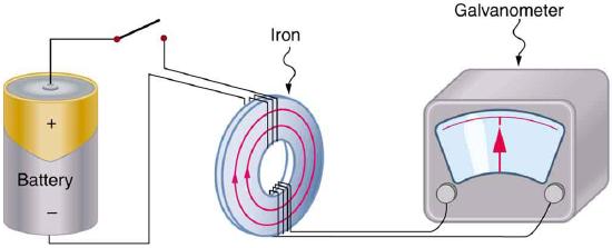
    The apparatus used by Faraday to demonstrate that magnetic fields can create currents is illustrated in Figure \(\PageIndex{1}\). When the switch is closed, a magnetic field is produced in the coil on the top part of the iron ring and transmitted to the coil on the bottom part of the ring. The galvanometer is used to detect any current induced in the coil on the bottom. It was found that each time the switch is closed, the galvanometer detects a current in one direction in the coil on the bottom. (You can also observe this in a physics lab.) Each time the switch is opened, the galvanometer detects a current in the opposite direction. Interestingly, if the switch remains closed or open for any length of time, there is no current through the galvanometer. Closing and opening the switch induces the current. It is the change in magnetic field that creates the current. More basic than the current that flows is the source voltage that causes it. The current is a result of an source voltage induced by a changing magnetic field, whether or not there is a path for current to flow.

    The picture shows Faraday’s apparatus for demonstrating that a magnetic field can produce a current. It consists of a cylinder shaped battery. The positive end of the battery is connected to an open switch. There is a ring shaped iron core consisting of a set of coils one on the top and another at the bottom. The other end of the switch is connected to one end of the top coil. The other end of the top coil is connected back to the battery. Both the ends of the bottom coil are shown connected across a galvanometer box which shows a null deflection.
    Figure \(\PageIndex{1}\): Faraday’s apparatus for demonstrating that a magnetic field can produce a current. A change in the field produced by the top coil induces a source voltage and, hence, a current in the bottom coil. When the switch is opened and closed, the galvanometer registers currents in opposite directions. No current flows through the galvanometer when the switch remains closed or open.

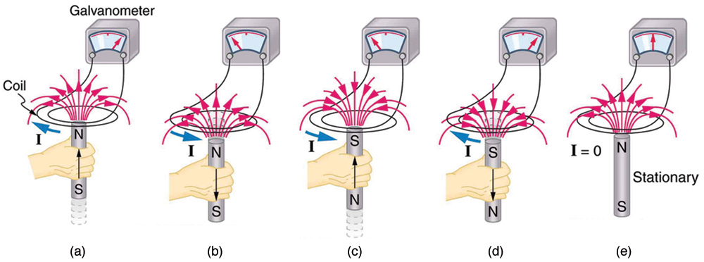
    An experiment easily performed and often done in physics labs is illustrated in Figure \(\PageIndex{2}\). A source voltage is induced in the coil when a bar magnet is pushed in and out of it. Source voltages of opposite signs are produced by motion in opposite directions, and the source voltages are also reversed by reversing poles. The same results are produced if the coil is moved rather than the magnet—it is the relative motion that is important. The faster the motion, the greater the source voltage, and there is no source voltage when the magnet is stationary relative to the coil.

    The diagram shows five stages of an experiment done by moving a magnet relative to a coil and measuring the e m f produced. The first stage of the experiment shows a wire coil with two loops connected across a galvanometer. The loop is in horizontal plane. A cylindrical rod shaped magnet is moved upward through the loop with the north pole of the magnet facing the loop and the South Pole away from the loop. The magnetic lines of force of the magnet are shown to emerge out from the North Pole and intersect the coil. A current is shown to be induced in the coil in clockwise direction. The galvanometer needle is shown to deflect toward right. The second stage of the experiment shows the next state of the first stage of the experiment. The cylindrical rod shaped magnet is now moved downward away from the loop with the north pole of the magnet facing the loop and South Pole away from the loop. The magnetic lines of force of the magnet are shown to emerge out from the North Pole and intersect the coil. A current is shown to be induced in the coil in anti clockwise direction. The galvanometer needle is shown to deflect toward left. The third stage of the experiment shows a wire coil with two loops connected across a galvanometer. The loop is in horizontal plane. A cylindrical rod shaped magnet is moved upward through the loop with the south pole of the magnet facing the loop and the North Pole away from the loop. The magnetic lines of force of the magnet are shown to merge into the South Pole and intersect the coil. A current is shown to be induced in the coil in anti clockwise direction. The galvanometer needle is shown to deflect toward left. The fourth stage of the experiment shows the next state of the third stage of the experiment. The cylindrical rod shaped magnet is now moved downward away from the loop with the south pole of the magnet facing the loop and the North Pole away from the loop. The magnetic lines of force of the magnet are shown to merge into the South Pole and intersect the coil. A current is shown to be induced in the coil in clockwise direction. The galvanometer needle is shown to deflect toward right. The fifth stage of the experiment shows a wire coil with two loops connected across a galvanometer. The loop is in horizontal plane. A cylindrical rod shaped magnet is held stationary near the loop with the north pole of the magnet facing the loop and south away from the loop. The magnetic lines of force of the magnet are shown to emerge out from the North Pole and intersect the coil. No current is induced in the coil. The galvanometer needle does not deflect.
    Figure \(\PageIndex{2}\): Movement of a magnet relative to a coil produces source voltages as shown. The same source voltages are produced if the coil is moved relative to the magnet. The greater the speed, the greater the magnitude of the source voltage, and the source voltage is zero when there is no motion.

    This page titled 9.1: Introduction is shared under a CC BY 4.0 license and was authored, remixed, and/or curated by OpenStax via source content that was edited to the style and standards of the LibreTexts platform.