6.1: Angular Momentum

Back in Chapter 2 we introduced the momentum of an object moving in one dimension as \(p = mv\), and found that it had the interesting property of being conserved in collisions between objects that made up an isolated system. Critical to that discussion was the idea that objects are represented by points, so they have well-defined positions. Of course, in real life, objects are not made up a single points, but are extended. We now want to move the discussion into studying these extended objects, that have real size, and understand how they transfer momentum differently than simple points. The biggest difference between points and extended objects it that extended objects can rotate, as well as move through space.

We want to define a quantity that measures this rotation, in the same way linear momentum measured something about how particles translated in space. This quantity is going to be angular momentum \(\vec{L}\), which we define as

\[\vec{L}=I\vec{\omega}\]

The variables here are the rotational analogues of the linear quantities; \(\vec{\omega}\) is angular velocity (like linear velocity \(\vec{v}\)), and \(I\) is called the moment of inertia, and is analogous to the mass \(m\). In this section we will build up an understanding of each of these quantities, and how they can be used to solve problems dealing with the rotation of extended objects.

The equation above is a vector, so we need to understand it's direction. It's tempting to say "the object rotates counterclockwise" or the like, but is there a vector direction associated to "counterclockwise"? There is, but it's probably not what you're thinking! The direction of counterclockwise (or clockwise) rotation comes from the right hand rule. The most basic version of the right hand rule is shown in the figure below, and the way you use it is:

1. Take your right hand...
2. ...curl the fingers of your right hand in the direction of rotation...
3. ...your thumb points in the direction of \(\vec{\omega}\).

 

                                                                                                  

Figure \(\PageIndex{1}\): From the Wikipedia page on this topic. In this case, the arrow along the hand shows the direction of \(\vec{\omega}\), and we might say "the angular velocity is directed up and to the right".

The angular velocity \(\vec{\omega}\) is the exact analog to the linear velocity \(\vec{v}\), although it deserves a little bit of attention. The unit for the angular velocity is angular distance per unit time, and in SI units that's radians per second. What's interesting about this is that for a single object, every point on the object will have the same angular velocity. It really has to be that way - if a hoop is spinning at two revolutions per second, asking what angular speed the outside of the hoop is spinning at had better be the same as every other point. Said another way, if any point on the object is spinning at a different rate (say, one revolution per second), that means the object is tearing itself apart! Those kinds of objects are more complicated, so we will always assume our object are rigid, meaning the entire object rotates at the same rate.

Now let's look at the newest aspect of this formula, the moment of inertia \(I\). Like the mass, this quantity encodes the inertia of an object, but includes information about it's shape. Specifically, for an object made up of a bunch of masses \(m_i\) which are located at distances \(r_i\) from an axis of rotation, the moment of inertia is

\[I=\sum_i m_i r_i^2.\label{eq:MomInert}\]

That looks like a simple formula, but if the shape is complicated, that sum might actually be very difficult or impossible to do¹. Fortunately, there are simplier expressions for many of the shapes we often encounter in nature. Many of these shapes are shown in the figure below, and many more can be found in Wikipedia.

                                                        

Table \(\PageIndex{1}\)

In nearly all of these examples (save those that have multiple different dimensions, like the annulus and the slab), the moment of inertia can be written like

\[I=\alpha MR^2,\]

where \(\alpha=1/2\) for a cylinder (or disk), \(\alpha=1\) for a hoop, etc.

Just like with linear momentum, we have a conservation principle associated with angular momentum:

Law of Conservation of Angular Momentum

The total angular moment of a closed system is conserved:

\[\sum_j \vec{L}_j=constant.\leftrightarrow \Delta \vec{L}=0\]

In addition, we have all the conditions around using this law that we had for conservation of linear momentum; namely, that the system must be isolated.

Adding Moments of Inertia

Just like the case of linear momentum, the total angular momentum of a system can be found by simply adding up the angular momenta of the individual parts of a system. For example, if object 1 is a spinning hoop (of mass \(M\) and radius \(R\), spinning at \(\omega_1\)), and object 2 is a spinning cylinder (of mass \(m\) and radius \(r\), spinning at \(\omega_2\)), then looking at the figure above we can write the total angular momentum of that system as

\[L_{tot}=L_1+L_2=MR^2\omega_1 + \frac{1}{2}mr^2\omega_2.\]

Here, we are assuming the two objects are not moving together at all. But, it often happens that we want to know the angular momentum of a single object that is made up of shapes found in our figure. For example, see figure 6.3.3 in the examples section at the end of this chapter, which is two disks rotating together. In that case the two disks have the same radius \(R\), but one has three times the mass of the other (\(M\) and \(3M\)). If those two disks are rotating at the same rate, their angular momentum would be

\[L_{tot}=L_1+L_2=\frac{1}{2}MR^2\omega + \frac{1}{2}3MR^2\omega=\frac{1}{2}(M+3M)R^2\omega.\]

Notice this is the same result we would have gotten if we had simply added their moments of inertia together first:

\[I_{tot}=I_1+I_2=\frac{1}{2}MR^2 + \frac{1}{2}3MR^2 = \frac{1}{2}(M+3M)R^2 \rightarrow L_{tot}=I_{tot}\omega=\frac{1}{2}(M+3M)R^2\omega.\]

The lesson here is when adding moments of inertia, do not add their masses or radii together alone - add their moments of inertia.

For another concrete example, consider finding the angular momentum of a rod with a mass on the edge (shown below).

                                                                                                  

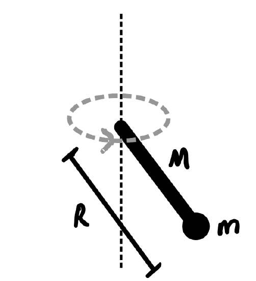
The total moment of inertia of this object is tricky, because the objects are different shapes. The rod has a moment of inertia of \(I_r=\frac{1}{3}MR^2\), while the point mass² had \(I_p=mR^2\). It's temping to just add the masses together, \(m+M\), but what fraction do you use out front, \(\frac{1}{3}\) or \(1\)? The answer is that you must add the moments of inertia themselves:

\[I_{tot}=I_r+I_p=\frac{1}{3}MR^2+mR^2=(\frac{1}{3}M+m)R^2.\]

Angular Speed vs Linear Speed

When objects rotate at a particular angular speed (in say, revolutions per second), the entire object moves at the same angular speed. This is because these objects are assumed to be rigid, so when one point on the objects goes around once, so does every other point. However, that doesn't mean that each of these points moves at the same linear speed (in say, meters per second). In fact, each point on the object moves at a different linear speed, depending on how far away it is from the center of rotation.

It's relatively easy to determine how these two quantities are related to each other, and this will turn out to be a very important formula. First, let's think about how fast a point a distance \(r\) from the center of an rotating object moves. If it takes a time period \(T\) for the object to rotate, such a point moves with speed

\[v=\frac{\text{distance traveled}}{\text{time interval}}=\frac{2\pi r}{T}.\]

Now, let's calculate the angular speed of this point (keeping in mind this is actually the angular speed of the entire object!). Over one rotation, it's angular speed will be

\[\omega=\frac{\text{angular distance traveled}}{\text{time interval}}=\frac{2\pi}{T}.\]

The \(2\pi\) here is just the number of radians the point travels for each rotation. These two formula are valid, but not that interesting because we don't know what the particular time period is here - so let's use the two of them to eliminate the time interval \(T\). Solving the second gives \(T=2\pi / \omega\), so let's plug that into the first:

\[v=\frac{2\pi r}{2\pi / \omega}=\frac{2\pi r \omega}{2\pi}\rightarrow v=r\omega\label{eq:AngLinSpeed}.\]

This very simple formula will be very helpful later; for now, it can give us some insight into how these point move. For example, at a particular angular speed \(\omega\), objects closer to the axis of rotation (smaller \(r\)) will move slower (have smaller \(v\)), while objects farther from the axis of rotation (larger \(r\)) will move faster (have larger \(v\)). This seems counterintuitive, but can be understood by seeing that objects far from the axis of rotation have further to travel then objects closer to the center, and have to do it over the same period of time.

---

¹In your calculus class you will learn how to calculate this for a wide variety of shapes.

²The moment of inertia of a point mass is not found in the table above, but it's easy to see the answer by looking at equation \ref{eq:MomInert}; with only one point in the sum it becomes \(mr^2\). This can also be seen by thinking about what a point mass actually looks like when it's rotating - a hoop, which is in the table above.