9.4: Advanced Application- Springs and Collisions


- Last updated
- Oct 2, 2023
- Save as PDF

( \newcommand{\kernel}{\mathrm{null}\,}\)
Two Carts Colliding and Compressing a Spring
Unlike the discussion in the previous section, which considered a stationary spring and asked only questions about initial and final states, this example is intended to show you how one can use “energy methods” to solve for the actual motion of a relatively complicated system as a function of time. The system is the two carts colliding, one of them fitted with a spring, considered in Section 9.3. Although all the physics involved is straightforward, the math is at a higher level than you will be using this semester, so I’m presenting this here as a “curiosity” only.
First, recall the total kinetic energy for a collision problem can be written as K=Kcm+Kconv, where (if the system is isolated) Kcm remains constant throughout. Then, the total mechanical energy E=K+U=Kcm+Kconv+U. This is also constant, and before the interaction happens, when U = 0, we have E=Kcm+Kconv,i, so setting these two things equal and canceling out Kcm we get
Kconv=Kconv,i−U
where the potential energy function is given by Equation (9.2.2). Introducing the relative coordinate x12=x2−x1, and the relative velocity v12, Equation (???) becomes
12μv212=12μv212,i−12k(x12−x0)2
an equation that must hold while the interaction is going on. We can solve this for v12, and then notice that both x12 and v12 are functions of time, and the latter is the derivative with respect to time of the former, so
v12=±√v212,i−(k/μ)(x12−x0)2
dx12dt=±√v212,i−(k/μ)(x12(t)−x0)2.
(The “±” sign means that the quantity on the right-hand side has to be negative at first, when the carts are coming together, and positive later, when they are coming apart. This is because I have assumed cart 1 starts to the left of cart 2, so going in cart 2, as seen from cart 1, appears to be moving to the left.)
Equation (???) is what is known, in calculus, as a differential equation. The problem is to find a function of t, x12(t), such that when you take its derivative you get the expression on the right-hand side. If you know how to calculate derivatives, you can check that the solution is in fact
x12(t)=x0−v12,iωsin[ω(t−tc)] for tc≤t≤tc+π/ω
where the quantity ω=√k/μ, and the time tc is the time cart 1 first makes contact with the spring: tc=(x2i−x0−x1i)/v1i. The solution (???) is valid for as long as the spring is compressed, which is to say, for as long as x12(t)<x0, or sin[ω(t−tc)]>0, which translates to the condition on t shown above.
Having a solution for x12, we could now obtain explicit results for x1(t) and x2(t) separately, using the fact that x1=xcm−m2x12/(m1+m2), and x2=xcm+m1x12/(m1+m2) (compare Eqs. (4.2.1), in chapter 4), and finding the position of the center of mass as a function of time is a trivial problem, since it just moves with constant velocity.
We do not, however, need to do any of this in order to generate the plots of the kinetic and potential energy shown in Figure 8.2.1: the potential energy depends only on x2−x1, which is given explicitly by Equation (???), and the kinetic energy is equal to Kcm+Kconv, where Kcm is constant and Kconv is given by Equation (???), which can also be easily rewritten in terms of Equation (???). The results are Eqs. (9.2.3) in the text.
Getting the Potential Energy Function from Collision Data
Consider the collision illustrated in Figure 4.3.1. Can we tell what the potential energy function is for the interaction between the two carts?
At first sight, it may seem that all the information necessary to “reconstruct” the function U(x1−x2) is available already, at least in graphical form: From Figure 4.3.1 you could get the value of x2−x1 at any time t; then from Figure 8.5.1 you can get the value of K (in the elastic-collision scenario) for the same value of t; and then you could plot U=E−K (where E is the total energy) as a function of x2−x1.
But there is a catch: Figure 4.3.1 shows that the colliding objects never get any closer than x2−x1 ≃ 0.28 mm, so we have no way to tell what U(x2−x1) is for smaller values of x2−x1. This is essentially the problem faced by particle physicists when they use collisions (which they do regularly) to try to determine the precise nature of the interactions between the particles they study!
You can check this for yourself. The functions I used for x1(t) and x2(t) in Figure 4.3.1 are
x1(t)=13((2t−10)erf(10−2t)+10erf(10)+t−e−4(t−5)2√π)−5x2(t)=13((5−t)erf(10−2t)−5erf(10)+t+e−4(t−5)22√π)
Here, “erf” is the so-called “error function,” which you can find in any decent library of mathematical functions. This looks complicated, but it just gives you the shapes you want for the velocity curves. The derivative of the above is
v1(t)=13(1+2erf(10−2t))v2(t)=13(1−erf(10−2t))
and you may want to try plotting these for yourself; the result should be Figure 4.3.1.
Now, assume (as I did for Figure 8.5.1) that m1 = 1 kg, and m2 = 2 kg, and use these values and the results of Eq (9.4.8) (assumed to be in m/s) to calculate Ksys as a function of t. Then U=Esys−Ksys, with Esys = 1/2 J:
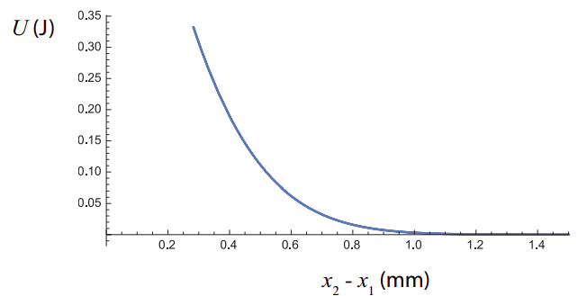
U=12−12m1v21(t)−12m2v22(t)=13(1−erf2(10−2t))
and now do a parametric plot of U versus x2−x1, using t as a parameter. You will end up with a figure like the one below: