24.2: Standing Waves and Resonance

Imagine you have a sinusoidal traveling wave of the form (12.1.5), only traveling to the left, incident from the right on a “fixed end” at \(x\) = 0. The incident wave will go as \(\xi_{0} \sin [2 \pi(x+c t) / \lambda]\); the reflected wave should be flipped left to right and upside down, so change \(x\) to \(−x\) and put an overall minus sign on the displacement, to get \(-\xi_{0} \sin [2 \pi(-x+c t) / \lambda]\). The sum of the two waves in the region \(x > 0\) is then

\[ \xi(x, t)=\xi_{0} \sin \left[\frac{2 \pi}{\lambda}(x+c t)\right]-\xi_{0} \sin \left[\frac{2 \pi}{\lambda}(-x+c t)\right]=2 \xi_{0} \sin \left(\frac{2 \pi x}{\lambda}\right) \cos (2 \pi f t) \label{eq:12.16} \]

using a trigonometrical identity for \(\sin(a + b)\), and \(f = c/\lambda\).

The result on the right-hand side of Equation (\ref{eq:12.16}) is called a standing wave. It does not travel anywhere, it just oscillates “in place”: every point x behaves like a separate oscillator with an amplitude \(2 \xi_{0} \sin (2 \pi x / \lambda)\). This amplitude is zero at special points, where \(2x/\lambda\) is equal to an integer. These points are called nodes.

We could think of “confining” a wave of this sort to a string fixed at both ends, if we make the string have an end at \(x\) = 0 and the other one at one of these points where the amplitude is zero; this means we want the length \(L\) of the string to satisfy

\[ 2L = n \lambda \label{eq:12.17} \]

where \(n\) = 1, 2,.... Alternatively, we can think of \(L\) as being fixed and Equation (\ref{eq:12.17}) as giving us the possible values of \(\lambda\) that will give us standing waves: \(\lambda = 2L/n\). Since \(f = c/\lambda\), we see that all these possible standing waves, for fixed \(L\) and \(c\), have different frequencies that we can write as

\[ f_{n}=\frac{n c}{2 L}, \quad n=1,2,3, \ldots \label{eq:12.18} .\]

Note that these are all multiples of the frequency \(f_1 = c/2L\). We call this the fundamental frequency of oscillation of a string fixed at both ends. The period corresponding to this fundamental frequency is the roundtrip time of a wave pulse around the string, \(2L/c\).

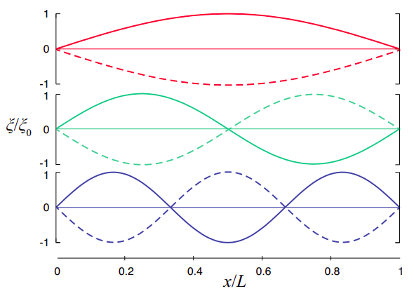
The first three standing waves are plotted in Figure \(\PageIndex{1}\). Their wave functions are given by the right-hand side of Equation (\ref{eq:12.16}), for 0 ≤ \(x\) ≤ \(L\), with \(\lambda = 2L/n\) (\(n\) = 1, 2, 3), and \(f = f_n = nc/2L\). The amplitude is arbitrary; in the figure I have set it equal to 1 for convenience. Calling the corresponding function \(u_n(x, t)\) is more or less common practice in other contexts:

\[ u_{n}(x, t)=\sin \left(\frac{n \pi x}{L}\right) \cos \left(2 \pi f_{n} t\right) \label{eq:12.19} .\]

These functions are called the normal modes of vibration of the string. In Figure \(\PageIndex{1}\) I have shown, for each of them, the displacement at the initial time, \(t\) = 0, as a solid line, and then half a period later as a dashed line. In addition to this, notice that the wave function vanishes identically (the string is flat) at the quarter-period intervals, \(t = 1/4f_n\) and \(t = 3/4f_n\). At those times, the wave has no elastic potential energy (since the string is unstretched): as with a simple oscillator passing through the equilibrium position, all its energy is kinetic. For \(n > 1\), there are also nodes (places where the oscillation amplitude is always zero) at points other than the ends. Including the endpoints, the \(n\)-th normal mode has \(n + 1\) nodes. The places where the oscillation amplitude is largest are called antinodes.

Figure \(\PageIndex{1}\): The three lowest-frequency normal modes of vibration of a string held down at both ends, corresponding to, from top to bottom, \(n\) = 1, 2, 3

Animations of these standing waves can be found in many places; one I particularly like is here: http://newt.phys.unsw.edu.au/jw/strings.html#standing. It also shows graphically how the standing wave can be considered as a superposition of two oppositely-directed traveling waves, as in Equation (\ref{eq:12.16}).

If we initially bent the string into one of the shapes shown in Figure \(\PageIndex{1}\), and then released it, it would oscillate at the corresponding frequency \(f_n\), keeping the same shape, only scaling it up and down by a factor \(\cos(2\pi f_{n}t)\) as time elapsed. So, another way to think of standing waves is as the natural modes of vibration of an extended system—the string, in this case, although standing waves can be produced in any medium that can carry a traveling wave.

What I mean by a “natural mode of vibration” is the following: a single oscillator, say, a pendulum, has a single “natural” frequency; if you displace it or hit it, it just oscillates at that frequency with a constant amplitude. An extended system, like the string, can be viewed as a collection of coupled oscillators, which may in general oscillate in many different and complicated ways; yet, there is a specific set of frequencies—for the string with two ends fixed, the sequence \(f_n\) of Equation (\ref{eq:12.18})—and associated shapes that will result in all the parts of the string performing simple harmonic motion, in synchrony, all at the same frequency.

Of course, to produce just one of these specific modes of oscillation requires some care (“driving” the string at the right frequency is probably the easiest way; see next paragraph); however, if you simply hit or pluck the string in any random way, a remarkable thing happens: the resulting motion will be, mathematically, described as a sum of sinusoidal standing waves, each with one of the frequencies \(f_n\), and each with a different amplitude \(A_n\). In a musical instrument, this will eventually generate a superposition of sound waves with frequencies \(f_1 = c/2L\), \(f_2 = 2f_1\), \(f_3 = 3f_1\) ... (called, in this context, the fundamental, \(f_1\), and its overtones, \(f_n = nf_1\)). Each one of these frequencies corresponds to a different pitch, or musical note, and the result will sound a little like a chord, although not nearly as pronounced—we will mostly hear only the fundamental, which corresponds to the root note of the chord, but all the notes in a major triad are in fact present in the vibration of a single guitar or piano string⁴.

But wait, there’s more! Suppose that you try to get the string to oscillate by “driving” it: that is to say, grabbing a hold of one end and shaking it at some frequency, only with a very small amplitude, so the displacement at that end remains always close to zero. In that case, you will typically get only very small amplitude oscillations, until the driving frequency hits one of the special frequencies \(f_n\), at which point you will get a large oscillation with the shape of the corresponding standing wave. This is a phenomenon known as resonance, and the \(f_n\) are the resonant frequencies of this system.

Note that the effect I just described is essentially the same as you experience when you are “pumping,” or simply pushing, a swing. Unless you do it at the right frequency, you do not get very far; but if you do it at the right frequency (which is the swing’s natural frequency, the one at which it will swing on its own), you can get huge amplitude oscillations. So, the frequencies (\ref{eq:12.18}) may be said to be the string’s natural oscillation frequencies in the same two ways: they are the ones at which it will oscillate if you just pluck it, and they are the ones at which you have to drive it if you want to get large oscillations.

Pretty much everything I have just shown you above for standing waves on a string applies to sound waves inside a tube or pipe open at both ends. In that case, however, it is not the displacement, but the pressure (or density) wave that must have zeros at the ends (since the ends are open, the pressure there must be just the average atmospheric pressure; note that the pressure or density waves in a sound wave do not give the absolute pressure or density, but the deviation, positive or negative, from the average). The math, however, is identical, and one finds the same set of normal modes and resonance frequencies as above. These are then the frequencies that would be produced when blowing in a flute or an organ pipe open at both ends. So, both from pipes and strings we get the same “harmonic series” of frequencies (\ref{eq:12.18}) that has been the foundation of Western music since at least the time of Pythagoras.

---

⁴It works like this: say \(f_1\) corresponds to a C, then \(f_2\) is the C above that, \(f_3\) the G above that, \(f_4\) the C above that, and \(f_5\) the E above that.