
24.5: Examples


- Last updated
- Jul 22, 2022
- Save as PDF

( \newcommand{\kernel}{\mathrm{null}\,}\)
Example 24.5.1: Displacement and Density/pressure in a longitudinal wave
The picture below shows the displacement of a medium (let’s say air) as a sound pulse travels through it. (Don’t worry about the units on the axes right now! We are only interested in qualitative results here.)
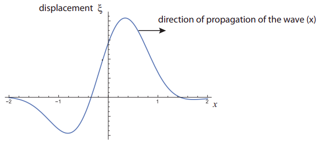
- Sketch the corresponding pressure (or density) pulse. Note: pressure and density are in phase, so one is large where the other is large. In either case what is always plotted is the difference between the actual pressure or density and the average pressure (for air, atmospheric pressure) or density of the medium.
- If this sound pulse is incident on water, sketch the reflected pulse, both in a displacement and in a pressure/density plot.
Solution
(a) The purpose of this example is to help refine the intuition you may have gotten from Figure 12.1.3 regarding the relationship between the displacement and the pressure/density in a longitudinal wave. When discussing Figure 12.1.3, I argued that the density should be high at a point like x=π in that figure, because the particles to the left of that point were being pushed to the right, and those to the right were being pushed to the left. However, a similar argument can be made to show that the density should be higher than its equilibrium value whenever the displacement curve has a negative slope, in general.
For instance, consider point x = 1 in the figure above. Particles both to the left and the right of that point are being pushed to the right (positive displacement), but the displacement is larger for the ones on the left, which will result in a bunching at x = 1.
Conversely, if you look at a point with positive slope, such as x = 0, you see that the particles on the right are pushed farther to the right than the particles on the left, which means the density around x = 0 will drop.
From this you may conclude that the density versus position graph will look somewhat like the negative of the derivative of the ξ-vs.-x graph: positive when ξ falls, negative when it rises, and zero at the “turning points” (maxima or minima of ξ(x)). This is, in fact, mathematically true, and is illustrated in the figure below.
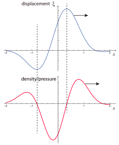
Figure24.5.1: Illustrating the relationship between displacement (blue curve) and pressure/density (red) in a longitudinal wave. The dashed lines separate the regions where the pressure (or density) is positive (higher than in the absence of the wave) from those where it is negative.
(b) If this sound wave is incident from air into water, it means it is going from a low impedance to a high impedance medium (both the density and the speed of sound are much greater in water than in air, giving a much larger Z=cρ0; see Equation (12.1.15) for the definition of impedance). This means the reflected displacement pulse will be flipped upside down, as well as left to right (see the figure on the next page). This is just (except for the scale, which here is arbitrary) like the bottom part of Figure 12.1.4.
However, if you now try to figure out the shape of the density/pressure wave based on the displacement wave, as we did in part (a), you’ll see that it is only reversed left to right, but not flipped upside down! This is a general property of longitudinal waves: the reflected pressure/density wave behaves in exactly the opposite way as the displacement wave, as far as the upside-down “flip” is concerned: it gets flipped when going from high impedance to low impedance, and not when going from low to high.
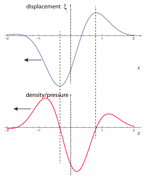
Figure 24.5.2: What the wave pulse in the previous figure would look like if reflected from a high-impedance medium. The displacement wave is reversed left to right and flipped upside down. The pressure/density wave is only reversed left to right.
If you are curious to see how this happens mathematically, the idea is that the density wave is proportional to −dξ/dx, and the reflected displacement wave goes like ξrefl=−ξinc(−x), where the first minus sign gives the vertical flip and the second the horizontal one. Taking the derivative of this last expression with respect to x then removes the minus sign in front.
Example 24.5.1: violin sounds
The “sounding length” of a violin string, from the bridge to the nut at the upper end of the fingerboard, is about 32 cm.
- If the string is tuned so that its fundamental frequency corresponds to a concert A (440 Hz), what is the speed of a wave on that string?
- If the string’s density is 0.66 g/m (note: the “g” stands for “grams”!), what is the tension on the string?
- When the string is played, its vibration is transmitted through the bridge to the violin plates. At what frequency will the plates vibrate?
- The vibration of the plates then sets up a sound wave in air. What is the wavelength of this wave?
Solution
(a) In Section 12.2 we saw that the fundamental frequency of a string fixed at both ends is f1=c/2L (corresponding to Equation (12.2.3) with n = 1). Setting this equal to 440 Hz, and solving for c,
c=2Lf1=2×(0.32m)×440s−1=282ms
(b) From Section 12.1, we have that the speed of a wave on a string is c=√Ft/μ, where Ft is the tension and μ the mass per unit length (Equation (12.1.11). Solving for Ft,
Ft=c2μ=(282ms)2×6.6×10−4kgm=52.5N
(c) The plates will vibrate at the same frequency as the string, 440 Hz, since they are driven by the motion of the string.
(d) The basic relationship to use here is Equation (12.1.4), f=c/λ, which we can solve for λ if we know c, the speed of sound in air. In Section 12.1 it was stated that the speed of sound in air is about 340 m/s, so we have
λ=cf=340m/s440s−1=0.77m