
8.2: The Biot-Savart Law
- Page ID
- 32218

\( \newcommand{\vecs}[1]{\overset { \scriptstyle \rightharpoonup} {\mathbf{#1}} } \)
\( \newcommand{\vecd}[1]{\overset{-\!-\!\rightharpoonup}{\vphantom{a}\smash {#1}}} \)
\( \newcommand{\id}{\mathrm{id}}\) \( \newcommand{\Span}{\mathrm{span}}\)
( \newcommand{\kernel}{\mathrm{null}\,}\) \( \newcommand{\range}{\mathrm{range}\,}\)
\( \newcommand{\RealPart}{\mathrm{Re}}\) \( \newcommand{\ImaginaryPart}{\mathrm{Im}}\)
\( \newcommand{\Argument}{\mathrm{Arg}}\) \( \newcommand{\norm}[1]{\| #1 \|}\)
\( \newcommand{\inner}[2]{\langle #1, #2 \rangle}\)
\( \newcommand{\Span}{\mathrm{span}}\)
\( \newcommand{\id}{\mathrm{id}}\)
\( \newcommand{\Span}{\mathrm{span}}\)
\( \newcommand{\kernel}{\mathrm{null}\,}\)
\( \newcommand{\range}{\mathrm{range}\,}\)
\( \newcommand{\RealPart}{\mathrm{Re}}\)
\( \newcommand{\ImaginaryPart}{\mathrm{Im}}\)
\( \newcommand{\Argument}{\mathrm{Arg}}\)
\( \newcommand{\norm}[1]{\| #1 \|}\)
\( \newcommand{\inner}[2]{\langle #1, #2 \rangle}\)
\( \newcommand{\Span}{\mathrm{span}}\) \( \newcommand{\AA}{\unicode[.8,0]{x212B}}\)
\( \newcommand{\vectorA}[1]{\vec{#1}} % arrow\)
\( \newcommand{\vectorAt}[1]{\vec{\text{#1}}} % arrow\)
\( \newcommand{\vectorB}[1]{\overset { \scriptstyle \rightharpoonup} {\mathbf{#1}} } \)
\( \newcommand{\vectorC}[1]{\textbf{#1}} \)
\( \newcommand{\vectorD}[1]{\overrightarrow{#1}} \)
\( \newcommand{\vectorDt}[1]{\overrightarrow{\text{#1}}} \)
\( \newcommand{\vectE}[1]{\overset{-\!-\!\rightharpoonup}{\vphantom{a}\smash{\mathbf {#1}}}} \)
\( \newcommand{\vecs}[1]{\overset { \scriptstyle \rightharpoonup} {\mathbf{#1}} } \)
\( \newcommand{\vecd}[1]{\overset{-\!-\!\rightharpoonup}{\vphantom{a}\smash {#1}}} \)
\(\newcommand{\avec}{\mathbf a}\) \(\newcommand{\bvec}{\mathbf b}\) \(\newcommand{\cvec}{\mathbf c}\) \(\newcommand{\dvec}{\mathbf d}\) \(\newcommand{\dtil}{\widetilde{\mathbf d}}\) \(\newcommand{\evec}{\mathbf e}\) \(\newcommand{\fvec}{\mathbf f}\) \(\newcommand{\nvec}{\mathbf n}\) \(\newcommand{\pvec}{\mathbf p}\) \(\newcommand{\qvec}{\mathbf q}\) \(\newcommand{\svec}{\mathbf s}\) \(\newcommand{\tvec}{\mathbf t}\) \(\newcommand{\uvec}{\mathbf u}\) \(\newcommand{\vvec}{\mathbf v}\) \(\newcommand{\wvec}{\mathbf w}\) \(\newcommand{\xvec}{\mathbf x}\) \(\newcommand{\yvec}{\mathbf y}\) \(\newcommand{\zvec}{\mathbf z}\) \(\newcommand{\rvec}{\mathbf r}\) \(\newcommand{\mvec}{\mathbf m}\) \(\newcommand{\zerovec}{\mathbf 0}\) \(\newcommand{\onevec}{\mathbf 1}\) \(\newcommand{\real}{\mathbb R}\) \(\newcommand{\twovec}[2]{\left[\begin{array}{r}#1 \\ #2 \end{array}\right]}\) \(\newcommand{\ctwovec}[2]{\left[\begin{array}{c}#1 \\ #2 \end{array}\right]}\) \(\newcommand{\threevec}[3]{\left[\begin{array}{r}#1 \\ #2 \\ #3 \end{array}\right]}\) \(\newcommand{\cthreevec}[3]{\left[\begin{array}{c}#1 \\ #2 \\ #3 \end{array}\right]}\) \(\newcommand{\fourvec}[4]{\left[\begin{array}{r}#1 \\ #2 \\ #3 \\ #4 \end{array}\right]}\) \(\newcommand{\cfourvec}[4]{\left[\begin{array}{c}#1 \\ #2 \\ #3 \\ #4 \end{array}\right]}\) \(\newcommand{\fivevec}[5]{\left[\begin{array}{r}#1 \\ #2 \\ #3 \\ #4 \\ #5 \\ \end{array}\right]}\) \(\newcommand{\cfivevec}[5]{\left[\begin{array}{c}#1 \\ #2 \\ #3 \\ #4 \\ #5 \\ \end{array}\right]}\) \(\newcommand{\mattwo}[4]{\left[\begin{array}{rr}#1 \amp #2 \\ #3 \amp #4 \\ \end{array}\right]}\) \(\newcommand{\laspan}[1]{\text{Span}\{#1\}}\) \(\newcommand{\bcal}{\cal B}\) \(\newcommand{\ccal}{\cal C}\) \(\newcommand{\scal}{\cal S}\) \(\newcommand{\wcal}{\cal W}\) \(\newcommand{\ecal}{\cal E}\) \(\newcommand{\coords}[2]{\left\{#1\right\}_{#2}}\) \(\newcommand{\gray}[1]{\color{gray}{#1}}\) \(\newcommand{\lgray}[1]{\color{lightgray}{#1}}\) \(\newcommand{\rank}{\operatorname{rank}}\) \(\newcommand{\row}{\text{Row}}\) \(\newcommand{\col}{\text{Col}}\) \(\renewcommand{\row}{\text{Row}}\) \(\newcommand{\nul}{\text{Nul}}\) \(\newcommand{\var}{\text{Var}}\) \(\newcommand{\corr}{\text{corr}}\) \(\newcommand{\len}[1]{\left|#1\right|}\) \(\newcommand{\bbar}{\overline{\bvec}}\) \(\newcommand{\bhat}{\widehat{\bvec}}\) \(\newcommand{\bperp}{\bvec^\perp}\) \(\newcommand{\xhat}{\widehat{\xvec}}\) \(\newcommand{\vhat}{\widehat{\vvec}}\) \(\newcommand{\uhat}{\widehat{\uvec}}\) \(\newcommand{\what}{\widehat{\wvec}}\) \(\newcommand{\Sighat}{\widehat{\Sigma}}\) \(\newcommand{\lt}{<}\) \(\newcommand{\gt}{>}\) \(\newcommand{\amp}{&}\) \(\definecolor{fillinmathshade}{gray}{0.9}\)By the end of this section, you will be able to:
- Explain how to derive a magnetic field from an arbitrary current in a line segment
- Calculate magnetic field from the Biot-Savart law in specific geometries, such as a current in a line and a current in a circular arc
We have seen that mass produces a gravitational field and also interacts with that field. Charge produces an electric field and also interacts with that field. Since moving charge (that is, current) interacts with a magnetic field, we might expect that it also creates that field—and it does.
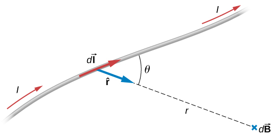
The equation used to calculate the magnetic field produced by a current is known as the Biot-Savart law. It is an empirical law named in honor of two scientists who investigated the interaction between a straight, current-carrying wire and a permanent magnet. This law enables us to calculate the magnitude and direction of the magnetic field produced by a current in a wire. The Biot-Savart law states that at any point \(P\) (Figure \(\PageIndex{1}\)), the magnetic field \(d\vec{B}\) due to an element \(d\vec{l}\) of a current-carrying wire is given by
\[d\vec{B} = \dfrac{\mu_0}{4 \pi} \dfrac{Id\vec{l} \times \hat{r}}{r^2}. \label{Biot-Savart law}\]
The constant \(\mu_0\) is known as the permeability of free space and is exactly
\[\mu_0 = 4\pi \times 10^{-7}\, T \cdot m/A \label{eq1}\]
in the SI system. The infinitesimal wire segment \(d\vec{l}\) is in the same direction as the current \(I\) (assumed positive), \(r\) is the distance from \(d\vec{l}\) to \(P\) and \(\hat{r}\) is a unit vector that points from \(d\vec{l}\) to \(P\), as shown in Figure \(\PageIndex{1}\). The direction of \(d\vec{B}\) is determined by applying the right-hand rule to the vector product \(d\vec{l} \times \hat{r}\). The magnitude of \(d\vec{B}\) is
\[dB = \dfrac{\mu_0}{4\pi} \dfrac{I \, dl \, \sin \, \theta}{r^2} \label{eq2}\]
where \(\theta\) is the angle between \(d\vec{l}\) and \(\hat{r}\). Notice that if \(\theta = 0\), then \(d\vec{B} = \vec{0}\). The field produced by a current element \(I d\vec{l}\) has no component parallel to \(d\vec{l}\).
The magnetic field due to a finite length of current-carrying wire is found by integrating Equation \ref{eq1} along the wire, giving us the usual form of the Biot-Savart law.
The magnetic field \(\vec{B}\) due to an element \(d\vec{l}\) of a current-carrying wire is given by
\[\vec{B} = \dfrac{\mu_0}{4\pi} \int_{wire} \dfrac{I \, d\vec{l} \times \hat{r}}{r^2}. \label{BS}\]
Since this is a vector integral, contributions from different current elements may not point in the same direction. Consequently, the integral is often difficult to evaluate, even for fairly simple geometries. The following strategy may be helpful.
To solve Biot-Savart law problems, the following steps are helpful:
- Identify that the Biot-Savart law is the chosen method to solve the given problem. If there is symmetry in the problem comparing \(\vec{B}\) and \(d\vec{l}\), Ampère’s law may be the preferred method to solve the question.
- Draw the current element length \(d\vec{l}\) and the unit vector \(\hat{r}\) noting that \(d\vec{l}\) points in the direction of the current and \(\hat{r}\) points from the current element toward the point where the field is desired.
- Calculate the cross product \(d\vec{l} \times \hat{r}\).The resultant vector gives the direction of the magnetic field according to the Biot-Savart law.
- Use Equation \ref{BS} and substitute all given quantities into the expression to solve for the magnetic field. Note all variables that remain constant over the entire length of the wire may be factored out of the integration.
- Use the right-hand rule to verify the direction of the magnetic field produced from the current or to write down the direction of the magnetic field if only the magnitude was solved for in the previous part.
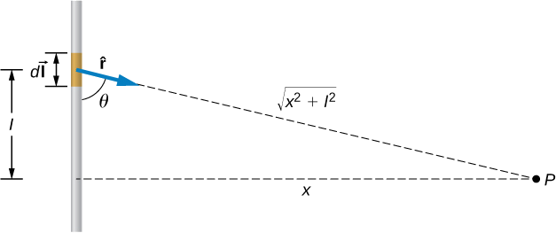
A short wire of length 1.0 cm carries a current of 2.0 A in the vertical direction (Figure \(\PageIndex{2}\)). The rest of the wire is shielded so it does not add to the magnetic field produced by the wire. Calculate the magnetic field at point P, which is 1 meter from the wire in the x-direction.
Strategy
We can determine the magnetic field at point \(P\) using the Biot-Savart law. Since the current segment is much smaller than the distance x, we can drop the integral from the expression. The integration is converted back into a summation, but only for small \(dl\), which we now write as \(\Delta l\). Another way to think about it is that each of the radius values is nearly the same, no matter where the current element is on the line segment, if \(\Delta l\) is small compared to x. The angle \(\theta\) is calculated using a tangent function. Using the numbers given, we can calculate the magnetic field at \(P\).
Solution
The angle between \(\Delta \vec{l}\) and \(\hat{r}\) is calculated from trigonometry, knowing the distances l and x from the problem:
\[\theta = \tan^{-1} \left(\dfrac{1 \, m}{0.01 \, m}\right) = 89.4^o. \nonumber\]
The magnetic field at point \(P\) is calculated by the Biot-Savart law (Equation \ref{eq2}):
\[\begin{align*} B &= \dfrac{\mu_0}{4\pi}\dfrac{I \Delta l \, \sin \, \theta}{r^2} \\[4pt] &= (1 \times 10^{-7} T \cdot m/A)\left( \dfrac{2 \, A(0.01 \, m)\, sin \, (89.4^o)}{(1 \, m)^2}\right) \\[4pt] &= 2.0 \times 10^{-9}T. \end{align*}\]
From the right-hand rule and the Biot-Savart law, the field is directed into the page.
Significance
This approximation is only good if the length of the line segment is very small compared to the distance from the current element to the point. If not, the integral form of the Biot-Savart law must be used over the entire line segment to calculate the magnetic field.
Using Example \(\PageIndex{1}\), at what distance would P have to be to measure a magnetic field half of the given answer?
Solution
1.41 meters
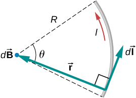
A wire carries a current I in a circular arc with radius R swept through an arbitrary angle \(\theta\) (Figure \(\PageIndex{3}\)). Calculate the magnetic field at the center of this arc at point P.
Strategy
We can determine the magnetic field at point P using the Biot-Savart law. The radial and path length directions are always at a right angle, so the cross product turns into multiplication. We also know that the distance along the path dl is related to the radius times the angle \(\theta\) (in radians). Then we can pull all constants out of the integration and solve for the magnetic field.
Solution
The Biot-Savart law starts with the following equation:
\[\vec{B} = \dfrac{\mu_0}{4\pi} \int_{wire} \dfrac{Id\vec{l} \times \hat{r}}{r^2}. \nonumber\]
As we integrate along the arc, all the contributions to the magnetic field are in the same direction (out of the page), so we can work with the magnitude of the field. The cross product turns into multiplication because the path \(dl\) and the radial direction are perpendicular. We can also substitute the arc length formula, \(dl = r\,d\theta\):
\[B = \dfrac{\mu_0}{4\pi} \int_{wire} \dfrac{Ir \, d\theta}{r^2}. \nonumber\]
The current and radius can be pulled out of the integral because they are the same regardless of where we are on the path. This leaves only the integral over the angle,
\[B = \dfrac{\mu_0I}{4\pi r} \int_{wire} d\theta.\nonumber\]
The angle varies on the wire from 0 to \(\theta\); hence, the result is
\[B = \dfrac{\mu_0I\theta}{4\pi r}. \nonumber\]
Significance
The direction of the magnetic field at point \(P\) is determined by the right-hand rule, as shown in the previous chapter. If there are other wires in the diagram along with the arc, and you are asked to find the net magnetic field, find each contribution from a wire or arc and add the results by superposition of vectors. Make sure to pay attention to the direction of each contribution. Also note that in a symmetric situation, like a straight or circular wire, contributions from opposite sides of point \(P\) cancel each other.
The wire loop forms a full circle of radius R and current I. What is the magnitude of the magnetic field at the center?
Solution
\(\dfrac{\mu_0 I}{2R}\)