13.4: Multiple-Slit Interference

Learning Objectives

By the end of this section, you will be able to:

• Describe the locations and intensities of secondary maxima for multiple-slit interference

Analyzing the interference of light passing through two slits lays out the theoretical framework of interference and gives us a historical insight into Thomas Young’s experiments. However, much of the modern-day application of slit interference uses not just two slits but many, approaching infinity for practical purposes. The key optical element is called a diffraction grating, an important tool in optical analysis, which we discuss in detail in chapter on Diffraction. Here, we start the analysis of multiple-slit interference by taking the results from our analysis of the double slit (N=2) and extending it to configurations with three, four, and much larger numbers of slits.

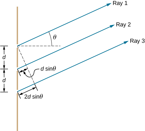
Figure $\PageIndex{1}$ shows the simplest case of multiple-slit interference, with three slits, or N=3. The spacing between slits is d, and the path length difference between adjacent slits is d sin θ, same as the case for the double slit. What is new is that the path length difference for the first and the third slits is 2d sin θ. The condition for constructive interference is the same as for the double slit, that is

$$d \sin θ=mλ \nonumber$$

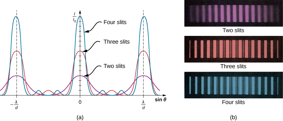
When this condition is met, 2d sin θ is automatically a multiple of λ, so all three rays combine constructively, and the bright fringes that occur here are called principal maxima. But what happens when the path length difference between adjacent slits is only λ/2? We can think of the first and second rays as interfering destructively, but the third ray remains unaltered. Instead of obtaining a dark fringe, or a minimum, as we did for the double slit, we see a secondary maximum with intensity lower than the principal maxima.

Figure $\PageIndex{1}$: Interference with three slits. Different pairs of emerging rays can combine constructively or destructively at the same time, leading to secondary maxima.

In general, for N slits, these secondary maxima occur whenever an unpaired ray is present that does not go away due to destructive interference. This occurs at (N−2) evenly spaced positions between the principal maxima. The amplitude of the electromagnetic wave is correspondingly diminished to 1/N of the wave at the principal maxima, and the light intensity, being proportional to the square of the wave amplitude, is diminished to $1/N^2$ of the intensity compared to the principal maxima. As Figure $\PageIndex{2}$ Interference fringe patterns for two, three and four slits. As the number of slits increases, more secondary maxima appear, but the principal maxima shows, a dark fringe is located between every maximum (principal or secondary). As N grows larger and the number of bright and dark fringes increase, the widths of the maxima become narrower due to the closely located neighboring dark fringes. Because the total amount of light energy remains unaltered, narrower maxima require that each maximum reaches a correspondingly higher intensity.

Figure $\PageIndex{2}$: Interference fringe patterns for two, three and four slits. As the number of slits increases, more secondary maxima appear, but the principal maxima become brighter and narrower. (a) Graph and (b) photographs of fringe patterns.