9.9: Linear and Rotational Quantities
- Last updated
- Jan 14, 2019
- Save as PDF
- Page ID
- 16990
( \newcommand{\kernel}{\mathrm{null}\,}\)
learning objectives
- Derive uniform circular motion from linear equations
Defining Circular Motion
The description of circular motion is described better in terms of angular quantity than its linear counter part. The reasons are easy to understand. For example, consider the case of uniform circular motion. Here, the velocity of particle is changing – though the motion is “uniform”. The two concepts do not go together. The general connotation of the term “uniform” indicates “constant”, but the velocity is actually changing all the time.

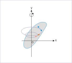
A Rotating Body: Each particle constituting the body executes a uniform circular motion about the fixed axis. For the description of the motion, angular quantities are the better choice.
When we describe the uniform circular motion in terms of angular velocity, there is no contradiction. The velocity (i.e. angular velocity) is indeed constant. This is the first advantage of describing uniform circular motion in terms of angular velocity.
Second advantage is that angular velocity conveys the physical sense of the rotation of the particle as against linear velocity, which indicates translational motion. Alternatively, angular description emphasizes the distinction between two types of motion (translational and rotational).
Relationship Between Linear and Angular Speed
For simplicity, let’s consider a uniform circular motion. For the length of the arc subtending angle ” at the origin and “r” is the radius of the circle containing the position of the particle, we have s=rθ.
Differentiating with respect to time, we have
dsdt=drdtθ+rdθdt.
Because drdt=0 for a uniform circular motion, we get v=ωr. Similarly, we also get a=αr where a stands for linear acceleration, while α refers to angular acceleration (In a more general case, the relationship between angular and linear quantities are given asv=ω×r,a=α×r+ω×v
Rotational Kinematic Equations
With the relationship of the linear and angular speed/acceleration, we can derive the following four rotational kinematic equations for constant aa and αα:
ω=ω0+αt:v=v0+atθ=ω0t+(12)αt2:x=v0t+(12)at2ω2=ω20+2αθ:v2=v20+2ax
Mass, Momentum, Energy, and Newton’s Second Law
As we use mass, linear momentum, translational kinetic energy, and Newton’s 2nd law to describe linear motion, we can describe a general rotational motion using corresponding scalar/vector/tensor quantities:
- Mass/ Rotational inertia:
- Linenar/angular momentum:
- Force/ Torque:
- Kinetic energy:
For example, just as we use the equation of motion F=maF=ma to describe a linear motion, we can use its counterpart τ=dLdt=r×F to describe an angular motion. The descriptions are equivalent, and the choice can be made purely for the convenience of use.
Key Points
- As we use mass, linear momentum, translational kinetic energy, and Newton’s 2nd law to describe linear motion, we can describe a general rotational motion using corresponding scalar/vector/tensor quantities.
- Angular and linear velocity have the following relationship: v=ω×r.
- As we use the equation of motion F=ma to describe a linear motion, we can use its counterpart τ=dLdt=r×F, to describe angular motion. The descriptions are equivalent, and the choice can be made purely for the convenience of use.
Key Items
- uniform circular motion: Movement around a circular path with constant speed.
- torque: A rotational or twisting effect of a force; (SI unit newton-meter or Nm; imperial unit foot-pound or ft-lb)
- rotational inertia: The tendency of a rotating object to remain rotating unless a torque is applied to it.
LICENSES AND ATTRIBUTIONS
CC LICENSED CONTENT, SHARED PREVIOUSLY
- Curation and Revision. Provided by: Boundless.com. License: CC BY-SA: Attribution-ShareAlike
CC LICENSED CONTENT, SPECIFIC ATTRIBUTION
- Sunil Kumar Singh, Circular Motion and Rotational Kinematics. September 17, 2013. Provided by: OpenStax CNX. Located at: http://cnx.org/content/m14014/latest/. License: CC BY: Attribution
- Boundless. Provided by: Boundless Learning. Located at: www.boundless.com//physics/definition/uniform-circular-motion. License: CC BY-SA: Attribution-ShareAlike
- torque. Provided by: Wiktionary. Located at: en.wiktionary.org/wiki/torque. License: CC BY-SA: Attribution-ShareAlike
- Boundless. Provided by: Boundless Learning. Located at: www.boundless.com//physics/definition/rotational-inertia. License: CC BY-SA: Attribution-ShareAlike
- Sunil Kumar Singh, Circular Motion and Rotational Kinematics. February 1, 2013. Provided by: OpenStax CNX. Located at: http://cnx.org/content/m14014/latest/. License: CC BY: Attribution

