
7.6: Contents of the Universe
- Page ID
- 47423
\( \newcommand{\vecs}[1]{\overset { \scriptstyle \rightharpoonup} {\mathbf{#1}} } \)
\( \newcommand{\vecd}[1]{\overset{-\!-\!\rightharpoonup}{\vphantom{a}\smash {#1}}} \)
\( \newcommand{\dsum}{\displaystyle\sum\limits} \)
\( \newcommand{\dint}{\displaystyle\int\limits} \)
\( \newcommand{\dlim}{\displaystyle\lim\limits} \)
\( \newcommand{\id}{\mathrm{id}}\) \( \newcommand{\Span}{\mathrm{span}}\)
( \newcommand{\kernel}{\mathrm{null}\,}\) \( \newcommand{\range}{\mathrm{range}\,}\)
\( \newcommand{\RealPart}{\mathrm{Re}}\) \( \newcommand{\ImaginaryPart}{\mathrm{Im}}\)
\( \newcommand{\Argument}{\mathrm{Arg}}\) \( \newcommand{\norm}[1]{\| #1 \|}\)
\( \newcommand{\inner}[2]{\langle #1, #2 \rangle}\)
\( \newcommand{\Span}{\mathrm{span}}\)
\( \newcommand{\id}{\mathrm{id}}\)
\( \newcommand{\Span}{\mathrm{span}}\)
\( \newcommand{\kernel}{\mathrm{null}\,}\)
\( \newcommand{\range}{\mathrm{range}\,}\)
\( \newcommand{\RealPart}{\mathrm{Re}}\)
\( \newcommand{\ImaginaryPart}{\mathrm{Im}}\)
\( \newcommand{\Argument}{\mathrm{Arg}}\)
\( \newcommand{\norm}[1]{\| #1 \|}\)
\( \newcommand{\inner}[2]{\langle #1, #2 \rangle}\)
\( \newcommand{\Span}{\mathrm{span}}\) \( \newcommand{\AA}{\unicode[.8,0]{x212B}}\)
\( \newcommand{\vectorA}[1]{\vec{#1}} % arrow\)
\( \newcommand{\vectorAt}[1]{\vec{\text{#1}}} % arrow\)
\( \newcommand{\vectorB}[1]{\overset { \scriptstyle \rightharpoonup} {\mathbf{#1}} } \)
\( \newcommand{\vectorC}[1]{\textbf{#1}} \)
\( \newcommand{\vectorD}[1]{\overrightarrow{#1}} \)
\( \newcommand{\vectorDt}[1]{\overrightarrow{\text{#1}}} \)
\( \newcommand{\vectE}[1]{\overset{-\!-\!\rightharpoonup}{\vphantom{a}\smash{\mathbf {#1}}}} \)
\( \newcommand{\vecs}[1]{\overset { \scriptstyle \rightharpoonup} {\mathbf{#1}} } \)
\(\newcommand{\longvect}{\overrightarrow}\)
\( \newcommand{\vecd}[1]{\overset{-\!-\!\rightharpoonup}{\vphantom{a}\smash {#1}}} \)
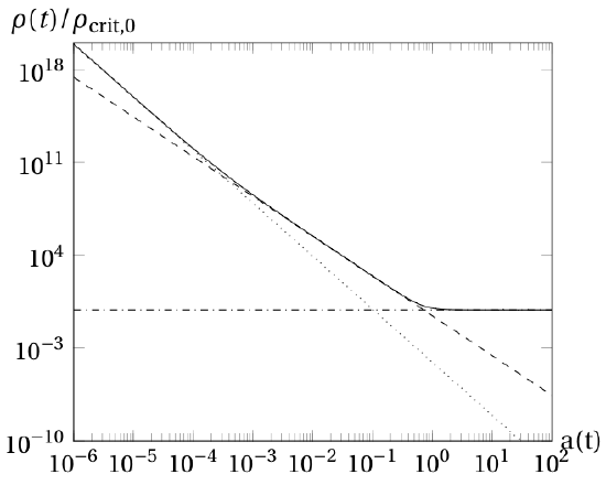
\(\newcommand{\avec}{\mathbf a}\) \(\newcommand{\bvec}{\mathbf b}\) \(\newcommand{\cvec}{\mathbf c}\) \(\newcommand{\dvec}{\mathbf d}\) \(\newcommand{\dtil}{\widetilde{\mathbf d}}\) \(\newcommand{\evec}{\mathbf e}\) \(\newcommand{\fvec}{\mathbf f}\) \(\newcommand{\nvec}{\mathbf n}\) \(\newcommand{\pvec}{\mathbf p}\) \(\newcommand{\qvec}{\mathbf q}\) \(\newcommand{\svec}{\mathbf s}\) \(\newcommand{\tvec}{\mathbf t}\) \(\newcommand{\uvec}{\mathbf u}\) \(\newcommand{\vvec}{\mathbf v}\) \(\newcommand{\wvec}{\mathbf w}\) \(\newcommand{\xvec}{\mathbf x}\) \(\newcommand{\yvec}{\mathbf y}\) \(\newcommand{\zvec}{\mathbf z}\) \(\newcommand{\rvec}{\mathbf r}\) \(\newcommand{\mvec}{\mathbf m}\) \(\newcommand{\zerovec}{\mathbf 0}\) \(\newcommand{\onevec}{\mathbf 1}\) \(\newcommand{\real}{\mathbb R}\) \(\newcommand{\twovec}[2]{\left[\begin{array}{r}#1 \\ #2 \end{array}\right]}\) \(\newcommand{\ctwovec}[2]{\left[\begin{array}{c}#1 \\ #2 \end{array}\right]}\) \(\newcommand{\threevec}[3]{\left[\begin{array}{r}#1 \\ #2 \\ #3 \end{array}\right]}\) \(\newcommand{\cthreevec}[3]{\left[\begin{array}{c}#1 \\ #2 \\ #3 \end{array}\right]}\) \(\newcommand{\fourvec}[4]{\left[\begin{array}{r}#1 \\ #2 \\ #3 \\ #4 \end{array}\right]}\) \(\newcommand{\cfourvec}[4]{\left[\begin{array}{c}#1 \\ #2 \\ #3 \\ #4 \end{array}\right]}\) \(\newcommand{\fivevec}[5]{\left[\begin{array}{r}#1 \\ #2 \\ #3 \\ #4 \\ #5 \\ \end{array}\right]}\) \(\newcommand{\cfivevec}[5]{\left[\begin{array}{c}#1 \\ #2 \\ #3 \\ #4 \\ #5 \\ \end{array}\right]}\) \(\newcommand{\mattwo}[4]{\left[\begin{array}{rr}#1 \amp #2 \\ #3 \amp #4 \\ \end{array}\right]}\) \(\newcommand{\laspan}[1]{\text{Span}\{#1\}}\) \(\newcommand{\bcal}{\cal B}\) \(\newcommand{\ccal}{\cal C}\) \(\newcommand{\scal}{\cal S}\) \(\newcommand{\wcal}{\cal W}\) \(\newcommand{\ecal}{\cal E}\) \(\newcommand{\coords}[2]{\left\{#1\right\}_{#2}}\) \(\newcommand{\gray}[1]{\color{gray}{#1}}\) \(\newcommand{\lgray}[1]{\color{lightgray}{#1}}\) \(\newcommand{\rank}{\operatorname{rank}}\) \(\newcommand{\row}{\text{Row}}\) \(\newcommand{\col}{\text{Col}}\) \(\renewcommand{\row}{\text{Row}}\) \(\newcommand{\nul}{\text{Nul}}\) \(\newcommand{\var}{\text{Var}}\) \(\newcommand{\corr}{\text{corr}}\) \(\newcommand{\len}[1]{\left|#1\right|}\) \(\newcommand{\bbar}{\overline{\bvec}}\) \(\newcommand{\bhat}{\widehat{\bvec}}\) \(\newcommand{\bperp}{\bvec^\perp}\) \(\newcommand{\xhat}{\widehat{\xvec}}\) \(\newcommand{\vhat}{\widehat{\vvec}}\) \(\newcommand{\uhat}{\widehat{\uvec}}\) \(\newcommand{\what}{\widehat{\wvec}}\) \(\newcommand{\Sighat}{\widehat{\Sigma}}\) \(\newcommand{\lt}{<}\) \(\newcommand{\gt}{>}\) \(\newcommand{\amp}{&}\) \(\definecolor{fillinmathshade}{gray}{0.9}\)If the universe is expanding, then the density will change with time. Furthermore, different components of the universe change their densities in different ways as the universe expands. These components can be broken into three general categories.
- Matter: Matter consists of particles whose mass is much greater than their kinetic energy. Stars, gas, neutrinos, and dark matter are all considered matter. As the universe expands, the density of matter goes down as the cube of the scale factor (since density of matter is inversely proportional to volume).
$$\begin{equation}
\rho_m(t)=\frac{\rho_{m,0}}{a^3(t)}\label{eq:MatterDensity}
\end{equation}$$
- Radiation: Radiation consists of particles whose mass is much less than their total energy. Today this category consists mostly of photons, but long ago neutrinos were a significant component. The density of radiation is inversely proportional to the fourth power of the scale factor. This is because, in addition to the effect of a scaling volume, the energy of radiation is also redshifted as the universe expands.
$$\begin{equation}
\rho_r(t)=\frac{\rho_{r,0}}{a^4(t)}\label{eq:RadiationDensity}
\end{equation}$$
- Dark Energy: Dark energy is something that hasn't been observed, and we don't know what it is. We introduce it as a component of the universe simply because it is required in order for the Friedmann equation to match current observations. Unlike matter and radiation, the density of dark energy is constant. As the universe expands, then, the total amount of dark energy increases.
$$\begin{equation}
\rho_\text{dark energy}\equiv \rho_\Lambda\sim 7\times 10^{-30}\frac{\text{g}}{\text{cm}^3}\label{eq:DarkEnergyDensity}
\end{equation}$$
The sum total of all of these represents the total density. Fig. 7.6.1 shows how each component, along with the total, evolves with the scale factor. Each component has a time in which it dominates over the others. At first the universe was radiation-dominated, then matter-dominated, and we are now in the transition point to the dark-energy-dominated regime.
In cosmology it is also convenient to define
$$\begin{equation}
\Omega_0=\frac{\rho(t_0)}{\rho_\text{crit,0}}.\label{eq:Omega0}
\end{equation}$$
If the current density is equal to the critical density, then this fraction is equal to 1. Meanwhile, \(\Omega_0>1\) for an overdense universe and \(\Omega_0<1\) for an underdense universe. Combining Eqs. \ref{eq:Omega0}, \ref{eq:MatterDensity}, \ref{eq:RadiationDensity}, and \ref{eq:DarkEnergyDensity} allows us to rewrite the Friedmann Equation (see Box 7.6.1) as
$$\begin{equation}
\dot{a}^2(t)=H_0^2\left(\frac{\Omega_{m,0}}{a(t)}+\frac{\Omega_{r,0}}{a^2(t)}+\Omega_\Lambda a^2(t)\right)-K\label{eq:FriedmannDimensionless}
\end{equation}
$$
This is a differential equation for \(a(t)\), meaning that if we have values for \(\Omega_{m,0}\), \(\Omega_{r,0}\), \(\Omega_\Lambda\), and \(K\), then we can determine \(a(t)\). Current observational experiments have constrained the values to
$$\begin{align}
\Omega_\text{m,0}&=0.27\pm 0.03\\
\Omega_\text{r,0}&=8.4\times 10^{-5}\\
\Omega_\Lambda&=0.73\pm 0.03.
\end{align}$$
Notice that the sum is indistinguishable from 1, which implies that the universe either has a flat geometry (\(K=0\)) or is very close to having a flat geometry. These numbers also make Equation \ref{eq:FriedmannDimensionless} impossible to solve by hand, which means that we have to solve it either numerically or by some other qualitative means. Fortunately, the equation is written in exactly the form needed to define an effective potential since it contains a kinetic-energy-like term (\(\dot{a}^2(t)\)) and a constant (\(-K\)). What remains is the effective potential.
$$\begin{equation}
V_\text{eff}(a)=-H_0^2\left(\frac{\Omega_{m,0}}{a(t)}+\frac{\Omega_{r,0}}{a^2(t)}+\Omega_\Lambda a^2(t)\right)\label{eq:UniverseEffectivePotential}
\end{equation}$$
Fig. 7.6.2 depicts a graph of the effective potential given current best estimates of \(\Omega_{m,0}=0.27\), \(\Omega_{r,0}\approx 0\), and \(\Omega_\Lambda=0.73\).
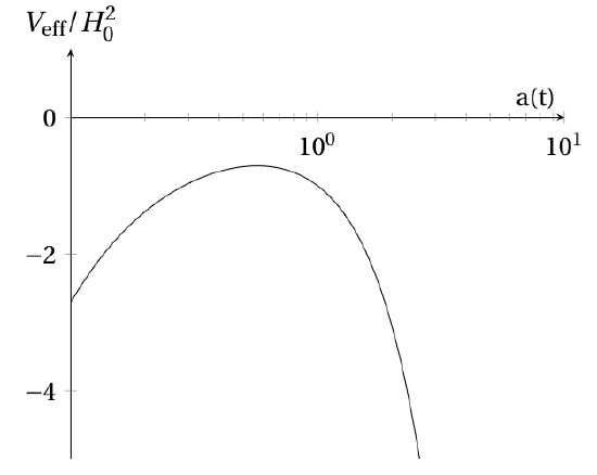
The "total energy" in the effective potential plot shown in Fig. 7.6.2 is a horizontal line at \(-K\). How are the different possible universes affected by the overall geometry of the universe? Assume that \(a(0)=0\).
- Answer
-
As usual with effective potential plots, I think it is helpful to imagine placing a marble on the graph and giving it a kick. If \(K=0\) or \(K<0\), the horizontal line depicting the "total energy" does not intersect the effective potential plot. This means that there are no turning points, so the marble will go over the hump and roll down the other side. In terms of the universe, this corresponds to the scale factor \(a(t)\) increasing without limit: an eternally expanding universe. If \(K\) is a sufficiently large positive number, however, then it will intersect the effective potential curve. Using our marble analogy, the marble would move to the right (corresponding to an increasing scale factor) but then would come to a stop at the turning point and roll back to the left. This represents a universe that initially expands but then eventually collapses on itself. This is referred to as the Big Crunch. We don't have to worry about that, however, since experimental observations indicate that \(K\approx 0\).
The lesson from the previous exercise is that it appears as though the universe will expand forever. As objects move farther and farther away from us, they eventually reach a point at which they are moving away from us faster than the speed of light. At that point, the light they emit will not be able to reach us, effectively removing them from the observable portion of the universe. As time goes on, the amount of stuff within the observable portion of the universe will get smaller and smaller. While the idea of a completely empty night sky may be sad, don't worry; our sun will be long dead by then.
The total density of the universe can be written as the sum of the densities of matter, radiation, and dark energy. Use this along with Eqs. \ref{eq:Omega0}, \ref{eq:MatterDensity}, \ref{eq:RadiationDensity}, and \ref{eq:DarkEnergyDensity} to derive Equation \ref{eq:FriedmannDimensionless}.
While Equation \ref{eq:FriedmannDimensionless} can't be solved by hand using the current observed values of the densities of each component, it can be solved in the case that the universe consists of only one of the three components. Here is the process, for example, if the universe is flat (\(K=0\)), consists only of radiation (\(\Omega_{r,0}=1\)), and starts with initial condition \(a(0)=0\).
$$\begin{align*}
\dot{a}^2(t)&=H_0^2\left(\frac{\cancelto{0}{\Omega_{m,0}}}{a(t)}+\frac{\cancelto{1}{\Omega_{r,0}}}{a^2(t)}+\cancelto{0}{\Omega_\Lambda} a^2(t)\right)-\cancelto{0}{K}&&\text{substitute values into Friedmann Equation}\\
\frac{da}{dt}&=\frac{H_0}{a}&&\text{take square root of both sides}\\
a\ da&=H_0\ dt&&\text{put all a's on one side and t's on the other}\\
\int\limits_{0}^{a(t)}a\ da&=\int\limits_{0}^{t}H_0\ dt&&\text{integrate both sides}\\
\frac{1}{2}a^2(t)-0&=H_0t-0&&\text{evaluate integral}\\
a(t)&=\sqrt{2H_0t}&&\text{solve for a(t)}
\end{align*}$$
Repeat this process to solve for \(a(t)\) for a flat universe that consists only of matter and for which \(a(0)=0\).
Repeat the process from the previous box to solve for \(a(t)\) for a flat universe that consists only of dark energy and for which \(a(0)=a_0\). Why can we not use \(a(0)=0\) in this case? (Explain both mathematically and physically.)