5.11: Solid-state NMR

In structural biology, X-ray crystallography, cryo-electron microscopy, and nuclear magnetic resonance (NMR) are the most useful tools to solve protein structures. However, when it comes to membrane proteins which are encoded in 20~30%¹ of most genomes, challenges appear. Since membrane proteins are embedded in the membrane and their structures and functions are highly dependent on their local bilayer lipid molecules, those environmental factors jeopardize the study of native membrane protein structures. Among all the known protein structures, only 1.7% ² are membrane proteins. For X-ray crystallography, the basic requirement to have a long-range order for diffraction means amphipathic molecules are required to align in the repetitive crystal lattice. Thus, it is not easy to obtain a large crystal of membrane protein which has a mixed protein topology. Cryo-electron microscopy is an emerging and promising technology to obtain high-resolution membrane protein structures ³. However, the cryogenic process for the sampling sacrifices the dynamic interaction of the protein and the bilayer components. The role of lipid phase is removed in the cryo-electron microscopic study of membrane proteins.

The well-established method of liquid-state nuclear magnetic resonance also suffers challenges when dealing with membrane proteins. In a typical liquid-state NMR experiment, a highly resolved spectrum is obtained due to the fast tumbling, or short correlation times (\(\tau_c\)), of molecules that average anisotropic interaction to zero. Only isotropic interaction with the external magnetic field such as scalar couplings remains that makes assigning peaks to individual nuclei and their neighbors possible. However, membrane protein must be embedded into detergent micelles, lipid bicelles, or lipid nanodiscs for liquid-state NMR.⁴ The large size of these vehicles dramatically increases the correlation time, thus anisotropic effect such as chemical shift anisotropy and through space dipolar coupling cannot be diminished. The non-averaged proton-proton dipolar interactions result in a featureless single broadband in the chemical shift that can span 25 kHz in width for proton NMR.⁵

Despite the disadvantage of anisotropy interaction in slow or non-tumbling molecules that leads to broad bands in NMR spectra, the broadband can be used to decode the anisotropic information of the molecules. In solid-state NMR (ssNMR), the anisotropic interactions in condensed phases including chemical shift anisotropy (CSA), internuclear dipolar coupling, quadrupolar interaction, and anisotropic J-coupling are studied.⁵ The sample size of solid-state NMR can vary from protein microcrystals⁶ to complexes like biofilms,⁷ intact membranes⁸ and even whole cells.⁹

Figure \(\PageIndex{1}\): Example of conformational analysis by using ssNMR¹⁰.

Chemical Shift Anisotropy

Electron surrounding the nucleus can shield the external magnetic field, disturb the Zeeman interaction, and lead to chemical shift. However, the electron cloud is not spherically distributed due to different bonding anisotropy. The anisotropy of a more asymmetrical functional group like the carbon of carbonyl is more significant than a symmetrical functional group like the carbon of methyl. Different orientations with respect to the applied external field, B ₀ , will have different chemical shift within the same nucleus and appear as a broadband. For example, the bandwidth, ∆ σ , of a broadband spectrum observed in unoriented phospholipid bilayer can correspond to ∆ σ = σ _‖ - σ _{⊥ ,} where σ _‖ is the chemical shift of bilayer oriented parallel to the external magnetic field and σ _⊥ is the chemical shift perpendicular to the external magnetic field. The ∆ σ encodes qualitative viscosity and specific orientation of the membrane molecule. This technique is frequently used to study membrane proteins made up of primarily transmembrane helices⁵.

Dipolar Interaction

Nuclei with spin greater than zero have a dipole moment. A nucleus with a dipole moment couples to another nucleus with nuclear spin I = ½ will appear as a doublet in the spectra. The splitting between two maxima can be calculated according to:

\[\Delta v_{D}(\alpha)=\frac{\mu_{0}}{4 \pi} \frac{\gamma_{i} \gamma_{j}}{r_{i j}^{3}} \frac{\mathrm{h}}{2 \pi^{2}}\left(\frac{3 \cos ^{2}(\alpha)-1}{2}\right) \label{eq10}\]

where μ ₀ is the permeability of vacuum, γ _i and γ _j are the gyromagnetic ratios of the nuclei, r _ij is the internuclear distance, h is the Planck’s constant, and α is the angle between the vector linking two nuclei and the external magnetic field, B ₀ . In a solid powder sample, each orientation of the dipolar interaction results in a set of doublet, by integrating every orientation, a Pake pattern will appear. If the internuclear distance remains the same but the molecule is fluctuating around an average angle, α ₀ , the equation should be rewritten as:

\[\Delta v_{D}\left(\alpha_{0}\right)=\frac{\mu_{0}}{4 \pi} \frac{\gamma_{i} \gamma_{j}}{r_{i j}^{3}} \frac{\mathrm{h}}{2 \pi^{2}}\left\langle\frac{3 \cos ^{2}(\alpha)-1}{2}\right\rangle \label{2}\]

where the term inside the brackets represents the probability distribution of the angle over the rapid fluctuations. The ∆ ν _D reflects internuclear distance, orientation and relative motion of a pair of nuclei, but each of the parameters needs to be determined independently in order to deduce the third parameter. The fluctuations of α around α ₀ can be minimized by cooling the sample, while internuclear distances can be determined from neutron diffraction measurements. In many cases, ∆ ν _D is very small and even difficult to measure.

Overall, the dipolar interaction of ¹³ C- ¹ H provides important information but is relatively weak comparing to ² H quadrupolar couplings⁵.

Quadrupolar Interaction

A quadrupolar moment exists when nucleus has spin I > 1/2. The quadrupolar interaction is strong and dominates the Zeeman effect. The most useful nucleus in membrane structure studies is ²H with I = 1. When a ²H bound to a ¹²C, the quadrupolar splitting ∆ ν _Q can be described as:

\[\Delta v_{Q}(\alpha)=\frac{3}{2} \chi_{Q}\left(\frac{3 \cos ^{2}(\alpha)-1}{2}\right) \label{3}\]

where χ _Q is the quadrupolar coupling constant and \(α\) is the angle between the vector linking two nuclei and the external magnetic field, B₀. In a fluidic membrane system, molecules can rotate around the bilayer normal very rapidly so that the effective averaged symmetry axis of the quadrupolar moment is parallel to the bilayer normal. The ∆ν_Q can be rewritten as:

\[\Delta v_{Q}(\beta)=\chi_{Q}\left\langle\frac{3 \cos ^{2}(\theta)-1}{2}\right\rangle\left(\frac{3 \cos ^{2}(\beta)-1}{2}\right) \label{eq4}\]

where \(β\) is the angle between the bilayer normal and the external magnetic field and θ is the instantaneous angle between the ¹² C- ² H bond and the bilayer normal as shown in Figure \(\PageIndex{2}\).

Figure \(\PageIndex{2}\): Definition of angles used in equations.

If the bilayer normal wobbles around an average angle β ₀ , the equation can be further derived as:

\[\Delta v_{Q}\left(\beta_{0}\right)=\chi_{Q}\left\langle\frac{3 \cos ^{2}(\theta)-1}{2}\right\rangle\left\langle\frac{3 \cos ^{2}(\beta)-1}{2}\right\rangle \label{eq5}\]

where the term inside the brackets represent the time average of the fluctuations and wobbling and is called the segmental order parameter \(S_{CD}\).

\[S_{C D}=\left\langle\frac{3 \cos ^{2}(\theta)-1}{2}\right\rangle\left\langle\frac{3 \cos ^{2}(\beta)-1}{2}\right\rangle= S_{fluc } S_{w o b} \label{eq6}\]

The ∆ ν _Q can be more complicated if the rapid motion of the quadrupolar moment does not have an axial symmetry, or if ¹⁴ N is involved in the quadrupolar interaction.

The line shape of the solid-state NMR provides orientational information. For slow motion with correlation time larger than 1/χ _Q , the linewidth will remain the same while the line shape is distorted. For fast motion such as sonicated membrane vesicles, the line shape can be narrow down to only one line.

Despite the important dynamic parameter \(S_{CD}\) can be obtained from the quadrupole splitting, the segmental order parameters in lipids cannot directly infer to the structural information. To obtain a complete average structure of a molecule, the whole order matrix, which contains nine elements, need to be determined. Without complete matrix, the spectra can only provide probabilities and boundaries of conformation in a model-independent fashion. That is why segmental order parameters in lipids are often stated in an elusive term such as ‘’probabilities of being in the trans conformation’⁵.

J-Coupling

J-coupling, or scalar coupling, is a through chemical bond isotropic interaction. It is an indirect dipole-dipole interaction mediated by the local electrons between two nuclear spins. J-coupling provides information about the connectivity of molecules, bond distance, and bond angles. The intensity of J-coupling is relatively weak compared to the anisotropic dipolar or quadrupolar interactions.

Magic-Angle Spinning

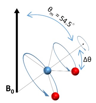
The most commonly used technique in solid-state NMR is Magic-Angle Spinning (MAS). It was proposed by E. R. Andrew, A. Bradbury, and R. G. Eades in 1958¹¹ , and by I. J. Lowe in 1959 ¹³ . Since the anisotropic interactions include the (\(3 \cos^2(θ) - 1\)) term, by spinning the sample at the angle θ = 54.74° where \(\cos^2 θ =1/3\) thus

\[3 \cos^2 ( θ ) - 1=0 ,\]

one can minimize both the anisotropic interactions and leave only the isotropic interaction. This angle is coined “Magic-Angle” and the method is termed “Magic-Angle Spinning” by Cornelis J. Gorter at the AMPERE congress in Pisa in 1960 ¹². The MAS can dramatically reduce the peak broadening due to anisotropic interaction and give a better resolution of the spectrum fur further analysis and identification of the structure.

By placing molecules at the angle of 54.74°, each bonding might have a different orientation, Δθ, with respect to the Magic-Angle, but after applying a rapid spinning around it, the orientation of all the dipolar moments will average to the Magic-Angle as shown in the following Figure.

Figure \(\PageIndex{3}\): Magic angle spinning to remove anisotropic interaction.

The spinning probe is propelled by air or nitrogen gases with the rotational frequency ranging from 1 to 130 kHz. When the spinning frequency is greater than the width of the static line, the chemical shift anisotropy can also be averaged to zero. The quadrupolar interaction is the strongest anisotropic interaction (170 kHz for ¹²C-²H bond¹⁴), therefore it requires a very high spinning frequency to remove the quadrupolar coupling, leaving only isotropic J-coupling in the spectra.

Sensitivity Enhancement

The sensitivity of solid-state NMR can be enhanced by varies techniques. Like the ordinary liquid phase NMR, a higher magnetic field can increase the Zeeman effect and increase the net magnetization due to Boltzmann distribution, thus increasing the sensitivity of NMR signal. Dynamic nuclear polarization (DNP) ¹⁵ is also a popular method in both liquid and solid-state NMR. The basic of DNP is very much similar to Nuclear Overhauser Effect (NOE) but the saturation transfer is from electron to nucleus rather than nucleus to nucleus in NOE. Since an unpaired electron is required to be saturated, a diradicals species must be presented near the target nucleus, thus spin-labelled experiments are often required to do the DNP enhancement. The cryoprobe is also a common technique in liquid-state NMR. The coil and signal preamplifier are cooled by liquid nitrogen or a stream of cold helium gas to reduce the electronics thermal noise and reach as much as a four-fold enhancement in signal-to-noise ratio¹⁶.

References

1. Piccoli, S.; Suku, E.; Garonzi, M.; Giorgetti, A., Genome-wide Membrane Protein Structure Prediction. Curr Genomics 2013, 14 (5), 324-9.
2. Hendrickson, W. A., Atomic-level analysis of membrane-protein structure. Nat Struct Mol Biol 2016, 23 (6), 464-7.
3. Abe, K.; Fujiyoshi, Y., Cryo-electron microscopy for structure analyses of membrane proteins in the lipid bilayer. Curr Opin Struct Biol 2016, 39, 71-78.
4. Wylie, B. J.; Do, H. Q.; Borcik, C. G.; Hardy, E. P., Advances in solid-state NMR of membrane proteins. Mol Phys 2016, 114 (24), 3598-3609.
5. Warschawski, D. E.; Traikia, M.; Devaux, P. F.; Bodenhausen, G., Solid-state NMR for the study of membrane systems: the use of anisotropic interactions. Biochimie 1998, 80 (5-6), 437-50.
6. Sperling, L. J.; Berthold, D. A.; Sasser, T. L.; Jeisy-Scott, V.; Rienstra, C. M., Assignment strategies for large proteins by magic-angle spinning NMR: the 21-kDa disulfide-bond-forming enzyme DsbA. J Mol Biol 2010, 399 (2), 268-82.
7. Cegelski, L., Bottom-up and top-down solid-state NMR approaches for bacterial biofilm matrix composition. J Magn Reson 2015, 253, 91-7.
8. Fu, R.; Wang, X.; Li, C.; Santiago-Miranda, A. N.; Pielak, G. J.; Tian, F., In situ structural characterization of a recombinant protein in native Escherichia coli membranes with solid-state magic-angle-spinning NMR. J Am Chem Soc 2011, 133 (32), 12370-3.
9. Rice, D. M.; Romaniuk, J. A.; Cegelski, L., Frequency-selective REDOR and spin-diffusion relays in uniformly labelled whole cells. Solid State Nucl Magn Reson 2015, 72, 132-9.
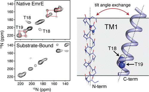
10. Cho MK, Gayen A, Banigan JR, Leninger M, Traaseth NJ., The Intrinsic Conformational Plasticity of Native EmrE Provides a Pathway for Multidrug Resistance. J Am Chem Soc 2014, 136, 8072-80.
11. Andrew, E. R.; Bradbury, A.; Eades, R. G., Nuclear Magnetic Resonance Spectra from a Crystal Rotated at High Speed. Nature 1958, 182 (4650), 1659-1659.
12. Lowe, I. J., Free Induction Decays of Rotating Solids. Phys Rev Lett 1959, 2 (7), 285-287.
13. Hennel, J. W.; Klinowski, J., Magic-angle spinning: a historical perspective. Top Curr Chem 2005, 246, 1-14.
14. Seelig, J., Deuterium magnetic resonance: theory and application to lipid membranes. Q Rev Biophys 1977, 10 (3), 353-418.
15. Griffin, R. G., High frequency dynamic nuclear polarization. Abstr Pap Am Chem S 2005, 229, U721-U721.
16. Griffiths, J., Solid-state NMR probes. Anal Chem 2008, 80 (5), 1381-1384.