1.10: The Friedmann Equation

Sticking with our Newtonian expanding universe, we will now derive the Friedmann equation that relates the mass/energy density to the rate of change of the scale factor.

We will proceed by using the Newtonian concept of energy conservation. (You may be surprised to hear me call this a Newtonian concept, but the fact is that energy conservation does not fully survive the transition from Newton to Einstein).

Box \(\PageIndex{1}\)

Assume the universe is filled with a fluid with mass density \(\rho\), that is flowing in a manner consistent with Hubble's law. Consider a test particle of mass \(m\) a distance \(a(t)\ell\) away from the origin of the coordinate system, that moves along with the fluid; i.e., all of its motion relative to the origin is due to the changing of the scale factor. We take the origin of the coordinate system to be at rest.

Exercise 10.1.1: Express the test particle's kinetic energy as a function of \(\dot a, \ell\) and \(m\).

Answer

K.E. is \(\frac{1}{2}mv^2\), where \(v = \dot a \ell\), so the test particle's kinetic energy is

\[\begin{equation*}
\begin{aligned}
\frac{1}{2}m\dot a^2 \ell ^2
\end{aligned}
\end{equation*}\]

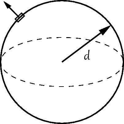
Exercise 10.1.2: Calculate the test particle's potential energy. Do so by considering just the mass interior to a sphere centered on the origin, with radius \(a(t)\ell\), as is justified for spherical mass distributions in Newtonian mechanics.

Answer

P.E. is \(-\frac{GM(<d)m}{d}\), where by \(M(<d)\) we mean the mass contained in the sphere of radius \(d\), so \(M(<d) = \frac{4}{3}\pi d^3 \rho.\)

Therefore the test particle's potential energy is

\[\begin{equation*}
\begin{aligned}
-G \frac{4}{3} \pi \rho d^2 m
\end{aligned}
\end{equation*}\]

Exercise 10.1.3: Add these two together and set them equal to a constant. Call the constant \(\kappa\).

Answer

\[\begin{equation*}
\begin{aligned}
\frac{1}{2}m\dot a^2 \ell ^2 - G \frac{4}{3} \pi \rho d^2 m = \kappa
\end{aligned}
\end{equation*}\]

Exercise 10.1.4: Manipulate your equation from Exercise 11.1.3 to get:

\[\begin{equation*}
\begin{aligned}
\left(\frac{\dot a}{a}\right)^2 = \frac{8\pi G \rho}{3} + \frac{2\kappa}{ml^2} \times \frac{1}{a^2}
\end{aligned}
\end{equation*}\]

Answer

Recall that \(d = a \ell \; \Longrightarrow \; \ell = \frac{d}{a}\), substituting this in and rearranging our equation we get

\[\begin{equation*}
\begin{aligned}
\frac{1}{2}md^2 \frac{\dot a^2}{a^2} - \frac{1}{2}md^2 \frac{8\pi G\rho}{3} = \kappa
\end{aligned}
\end{equation*}\]

dividing through by \(\frac{1}{2}md^2\) gives

\[\begin{equation*}
\begin{aligned}
\frac{\dot a^2}{a^2} - \frac{8\pi G\rho}{3} = \frac{2\kappa}{m}\frac{1}{d^2}
\end{aligned}
\end{equation*}\]

Then we substitute back in \(d = a \ell\) and solve for \(\big(\frac{\dot a}{a}\big)^2\):

\[\begin{equation*}
\begin{aligned}
\left(\frac{\dot a}{a}\right)^2 = \frac{8\pi G \rho}{3} + \frac{2\kappa}{ml^2} \times \frac{1}{a^2}
\end{aligned}
\end{equation*}\]

Note that everything in that last term in front of the \(\frac{1}{a^2}\) factor is a constant in time. Because the other two terms in the equation are constant in space, we can conclude that the third term is also constant in space. Since \(\frac{1}{a^2}\) is also constant in space, the combination \(2\kappa/(ml^2)\) that precedes it must also be constant in space. We are free to simplify this term by introducing a new space-time constant that we will call \(-k\) so the Friedmann equation becomes:
\[\left(\frac{\dot a}{a}\right)^2 = \frac{8\pi G \rho}{3} - \frac{k}{a^2}.\]

In general relativity this constant, \(k\), is the same as the curvature constant in the FRW invariant distance equation. Of course we cannot use Newtonian physics to derive this fact, as curvature is a non-Newtonian concept. We simply state it here with no proof.

To fully have a handle on the dynamics, what's left is to determine how \(\rho\) changes as \(a\) changes, a subject we will address in the next few chapters. For now, to explore some consequences of the Friedmann equation, we assume \(\rho \propto a^{-3}\). This is a model that most cosmologists, over 25 years ago, thought was probably an excellent approximation to reality. With this assumption, there becomes a connection between the geometry of space, and the fate of the universe. If \(k > 0\) the expansion eventually halts and becomes contraction. If \(k < 0\) or if \( k =0\) the expansion rate remains positive, approaching but never reaching zero.

Note that the Friedmann equation gives us another means of inferring the curvature constant \(k\). All we need to do is determine the expansion rate today, \(H_0\) and the density of matter today, \(\rho_0\) and plug them in to the Friedmann equation and solve for \(k\). We've already seen, in principle, how to infer \(H_0\) by measuring luminosity distances and redshifts for objects at low redshift and using \(cz =H_0 d_{\rm lum}\). Measuring \(\rho_0 \), is trickier, and a subject we may not get to in this course. However, cosmologists have been attempting to measure \(\rho_0\) for decades, in order to then infer \(k\). Because they also used to believe \(\rho \propto a^{-3}\), this meant a density measurement could be used to infer the fate of the universe. This situation is the origin of the statement "density is destiny." As we will see, the surprising discovery of cosmic acceleration ( \( \ddot a > 0\) ) destroyed this notion.

HOMEWORK Problems

Note: Unless directed otherwise, in these first 3 problems assume that \(k = 0\) and \(\rho \propto a^{-3}\).

Problem \(\PageIndex{1}\)

1. What is the age of the universe as a function of \(H\)?
2. If there were some non-zero curvature, would the magnitude of its contribution to the expansion rate, relative to that of the energy density, increase or decrease over time?

Problem \(\PageIndex{2}\)

What is the furthest physical distance a signal could travel if it started at the beginning? Express your answer as a function of \(H\). To be clear, the distance I mean is the physical distance, at the time when the expansion rate is \(H\), between the particle's actual spatial location and the spatial location it would have had if it had been stationary since the beginning. 

Problem \(\PageIndex{3}\)

Is there any limit to the comoving distance we can send a signal, if we send one now and are willing to wait an arbitrarily long amount of time? This is equivalent to asking, are there galaxies out at sufficient distance, that a light signal we send to them now will never get to them, even given an infinite amount of time?

Problem \(\PageIndex{4}\)

Show that if \(\rho \propto a^{p} \) with \(p < -2\), then \(\ddot a < 0.\) Do not assume \(k = 0\).