
1.4: Superposition and Interference
- Page ID
- 27759

\( \newcommand{\vecs}[1]{\overset { \scriptstyle \rightharpoonup} {\mathbf{#1}} } \)
\( \newcommand{\vecd}[1]{\overset{-\!-\!\rightharpoonup}{\vphantom{a}\smash {#1}}} \)
\( \newcommand{\dsum}{\displaystyle\sum\limits} \)
\( \newcommand{\dint}{\displaystyle\int\limits} \)
\( \newcommand{\dlim}{\displaystyle\lim\limits} \)
\( \newcommand{\id}{\mathrm{id}}\) \( \newcommand{\Span}{\mathrm{span}}\)
( \newcommand{\kernel}{\mathrm{null}\,}\) \( \newcommand{\range}{\mathrm{range}\,}\)
\( \newcommand{\RealPart}{\mathrm{Re}}\) \( \newcommand{\ImaginaryPart}{\mathrm{Im}}\)
\( \newcommand{\Argument}{\mathrm{Arg}}\) \( \newcommand{\norm}[1]{\| #1 \|}\)
\( \newcommand{\inner}[2]{\langle #1, #2 \rangle}\)
\( \newcommand{\Span}{\mathrm{span}}\)
\( \newcommand{\id}{\mathrm{id}}\)
\( \newcommand{\Span}{\mathrm{span}}\)
\( \newcommand{\kernel}{\mathrm{null}\,}\)
\( \newcommand{\range}{\mathrm{range}\,}\)
\( \newcommand{\RealPart}{\mathrm{Re}}\)
\( \newcommand{\ImaginaryPart}{\mathrm{Im}}\)
\( \newcommand{\Argument}{\mathrm{Arg}}\)
\( \newcommand{\norm}[1]{\| #1 \|}\)
\( \newcommand{\inner}[2]{\langle #1, #2 \rangle}\)
\( \newcommand{\Span}{\mathrm{span}}\) \( \newcommand{\AA}{\unicode[.8,0]{x212B}}\)
\( \newcommand{\vectorA}[1]{\vec{#1}} % arrow\)
\( \newcommand{\vectorAt}[1]{\vec{\text{#1}}} % arrow\)
\( \newcommand{\vectorB}[1]{\overset { \scriptstyle \rightharpoonup} {\mathbf{#1}} } \)
\( \newcommand{\vectorC}[1]{\textbf{#1}} \)
\( \newcommand{\vectorD}[1]{\overrightarrow{#1}} \)
\( \newcommand{\vectorDt}[1]{\overrightarrow{\text{#1}}} \)
\( \newcommand{\vectE}[1]{\overset{-\!-\!\rightharpoonup}{\vphantom{a}\smash{\mathbf {#1}}}} \)
\( \newcommand{\vecs}[1]{\overset { \scriptstyle \rightharpoonup} {\mathbf{#1}} } \)
\(\newcommand{\longvect}{\overrightarrow}\)
\( \newcommand{\vecd}[1]{\overset{-\!-\!\rightharpoonup}{\vphantom{a}\smash {#1}}} \)
\(\newcommand{\avec}{\mathbf a}\) \(\newcommand{\bvec}{\mathbf b}\) \(\newcommand{\cvec}{\mathbf c}\) \(\newcommand{\dvec}{\mathbf d}\) \(\newcommand{\dtil}{\widetilde{\mathbf d}}\) \(\newcommand{\evec}{\mathbf e}\) \(\newcommand{\fvec}{\mathbf f}\) \(\newcommand{\nvec}{\mathbf n}\) \(\newcommand{\pvec}{\mathbf p}\) \(\newcommand{\qvec}{\mathbf q}\) \(\newcommand{\svec}{\mathbf s}\) \(\newcommand{\tvec}{\mathbf t}\) \(\newcommand{\uvec}{\mathbf u}\) \(\newcommand{\vvec}{\mathbf v}\) \(\newcommand{\wvec}{\mathbf w}\) \(\newcommand{\xvec}{\mathbf x}\) \(\newcommand{\yvec}{\mathbf y}\) \(\newcommand{\zvec}{\mathbf z}\) \(\newcommand{\rvec}{\mathbf r}\) \(\newcommand{\mvec}{\mathbf m}\) \(\newcommand{\zerovec}{\mathbf 0}\) \(\newcommand{\onevec}{\mathbf 1}\) \(\newcommand{\real}{\mathbb R}\) \(\newcommand{\twovec}[2]{\left[\begin{array}{r}#1 \\ #2 \end{array}\right]}\) \(\newcommand{\ctwovec}[2]{\left[\begin{array}{c}#1 \\ #2 \end{array}\right]}\) \(\newcommand{\threevec}[3]{\left[\begin{array}{r}#1 \\ #2 \\ #3 \end{array}\right]}\) \(\newcommand{\cthreevec}[3]{\left[\begin{array}{c}#1 \\ #2 \\ #3 \end{array}\right]}\) \(\newcommand{\fourvec}[4]{\left[\begin{array}{r}#1 \\ #2 \\ #3 \\ #4 \end{array}\right]}\) \(\newcommand{\cfourvec}[4]{\left[\begin{array}{c}#1 \\ #2 \\ #3 \\ #4 \end{array}\right]}\) \(\newcommand{\fivevec}[5]{\left[\begin{array}{r}#1 \\ #2 \\ #3 \\ #4 \\ #5 \\ \end{array}\right]}\) \(\newcommand{\cfivevec}[5]{\left[\begin{array}{c}#1 \\ #2 \\ #3 \\ #4 \\ #5 \\ \end{array}\right]}\) \(\newcommand{\mattwo}[4]{\left[\begin{array}{rr}#1 \amp #2 \\ #3 \amp #4 \\ \end{array}\right]}\) \(\newcommand{\laspan}[1]{\text{Span}\{#1\}}\) \(\newcommand{\bcal}{\cal B}\) \(\newcommand{\ccal}{\cal C}\) \(\newcommand{\scal}{\cal S}\) \(\newcommand{\wcal}{\cal W}\) \(\newcommand{\ecal}{\cal E}\) \(\newcommand{\coords}[2]{\left\{#1\right\}_{#2}}\) \(\newcommand{\gray}[1]{\color{gray}{#1}}\) \(\newcommand{\lgray}[1]{\color{lightgray}{#1}}\) \(\newcommand{\rank}{\operatorname{rank}}\) \(\newcommand{\row}{\text{Row}}\) \(\newcommand{\col}{\text{Col}}\) \(\renewcommand{\row}{\text{Row}}\) \(\newcommand{\nul}{\text{Nul}}\) \(\newcommand{\var}{\text{Var}}\) \(\newcommand{\corr}{\text{corr}}\) \(\newcommand{\len}[1]{\left|#1\right|}\) \(\newcommand{\bbar}{\overline{\bvec}}\) \(\newcommand{\bhat}{\widehat{\bvec}}\) \(\newcommand{\bperp}{\bvec^\perp}\) \(\newcommand{\xhat}{\widehat{\xvec}}\) \(\newcommand{\vhat}{\widehat{\vvec}}\) \(\newcommand{\uhat}{\widehat{\uvec}}\) \(\newcommand{\what}{\widehat{\wvec}}\) \(\newcommand{\Sighat}{\widehat{\Sigma}}\) \(\newcommand{\lt}{<}\) \(\newcommand{\gt}{>}\) \(\newcommand{\amp}{&}\) \(\definecolor{fillinmathshade}{gray}{0.9}\)Combining Similar Waves
When two or more waves of the same type in the same medium coexist in the same region of space, they combine to create a new wave. The way they combine is a simple process known as superposition. This consists of simply adding the displacements (or whatever the wave function represents) of the two or more waves at the same place and time. For a 1-dimensional wave, this means:
\[f_{tot}\left(x,t\right)=f_1\left(x,t\right)+f_2\left(x,t\right)\]
Alert
It's important to emphasize that two waves can only superpose if they are the same type. Many different kinds of waves can travel through the same medium (light, sound, and displacement waves can all travel through water in a lake, for instance), but these cannot superpose with each other.
It’s easy to show that if the two individual wave functions satisfy the wave equation, then so does the total wave function. It bears repeating with a diagram that this superposition sum involves adding displacements at the same place and time. So if we took a snapshot of two waves, we would determine the total wave by lining them up:
Figure 1.4.1 – Superposition
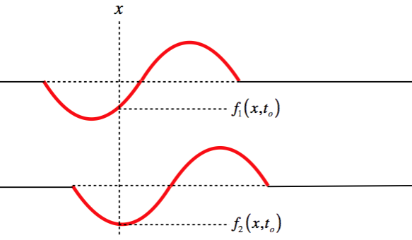
The composite wave is then the combination of all of the points added thus. Of course, these are traveling waves, so over time the superposition produces a composite wave that can vary with time in interesting ways. Here is a simple example of two pulses "colliding" (the "sum" of the top two waves yields the bottom wave).
Figure 1.4.2 – "Collision" of Pulses
Notice that even though the resultant wave looks very different from its "parents," the medium somehow "remembers" the original waves, and when they no longer coincide, they continue along as exactly the waves they were before the superposition. That is, the waves do not affect each other, as particles would if they collided – waves don't bounce off each other, for example. They simply create a new wave while they occupy the same space in the medium, and when their individual motions carry them to different parts of the medium, they return to being the waves they were before.
Interference – All-or-Nothing
There are some special cases involving superposition that are particularly interesting to examine, and these involve a phenomenon known as interference. There are many degrees of interference possible, all of which fall between the following two extremes:
- constructive interference: The waves are perfectly aligned and timed so that their crests and troughs coincide, such that the total wave has the maximum possible amplitude (equal to the sum of the amplitudes of the two constituent waves).
- destructive interference: The waves are perfectly aligned and timed so that the crests of one wave align with the troughs of the other such that leading to a wave that has the minimum possible amplitude (equal to the difference of the amplitudes of the two constituent waves).
The phrase total destructive interference refers to the case of destructive interference when the resultant wave has zero amplitude, i.e. the two waves totally cancel each other. In the cases we will discuss, we will only talk about this extreme case of destructive interference, so we will typically leave out the word “total,” even though we are still talking about total cancelation.
Interference – Intensity of Combined Wave
We will examine a great many examples of interference in physical phenomena in the sections to come. We therefore need to take some time to develop the mathematics behind this effect. We will do this within the same framework that we have been using – that of harmonic waves. When we look at the physical attributes of interference, what we will be examining is what happens to the intensity of the combined wave. For example, interference in sound will be exhibited in volume, and in light it will be brightness. Both of these are measures of intensity. We need a reference point for intensity, and the one we will use is that of maximal constructive interference. So what we seek is an equation that relates the intensity of two superposed, out-of-phase, but otherwise identical waves to the intensity we would see if they were in phase. That is, we want something that looks like this:
\[I\left(\Delta\Phi\right) = I_o g\left(\Delta\Phi\right) \]
The quantity \(I\) is the intensity of the wave as a function of the phase difference of the two (identical) parent waves. If the two waves happen to be in phase, then the combined wave's intensity is \(I_o\) when the two waves are in phase. Note that this is four times the intensity of each individual wave, since the constructive interference adds the amplitudes (which are equal – the waves are identical) and the intensity is proportional to the square of the amplitude.
The function needs to have the following properties:
- It has to always be non-negative, since intensity is never a negative number.
- It has to vanish when the phase difference equals \(\pi\) (modulo \(2\pi\)), since this means the waves totally destructively interfere.
- It has to equal 1 when when the phase difference is 0 (modulo \(2\pi\)), since this means the waves constructively interfere.
To find this function, we start with two wave functions that are identical except for their phases and superpose them:
We want this function to only depend upon the difference in the two phases, so we will write each total phase in terms of deviation from their average phase (which we will call simply \(\Phi\)), and the difference in phase between the two waves, \(\Delta\Phi\):
\[\Phi = \dfrac{\Phi_1+\Phi_2}{2}\;\;\;\Rightarrow\;\;\;\Phi_1=\Phi-\dfrac{\Delta\Phi}{2},\;\;\;\Phi_2=\Phi+\dfrac{\Delta\Phi}{2}\]
Plug these into Equation 1.4.3 gives:
\[f_{tot} = A\left[\cos\left(\Phi-\frac{\Delta \Phi}{2}\right) + \cos\left(\Phi+\frac{\Delta \Phi}{2}\right)\right]\]
Now we can apply a trigonometric identity:
The phase difference between the two waves can be written in terms of the difference in position, time, and the phase constant, using Equation 1.2.9:
As the waves propagate along, the values of \(x\) and \(t\) will change, but as the two waves are identical (traveling in the same direction with the same speed), the differences in \(x\) and \(t\) don’t change for a given phase. Therefore the factor in Equation 1.4.6 that includes the phase difference is a constant. Putting that constant together with the \(2A\) gives us the amplitude of the new conglomerate wave (with the time-varying phase being the average of the phases of the two waves):
The intensity is proportional to the square of the amplitude, so the intensity of this combined wave is:
\[I\propto A_{new}^2 = 4A^2\cos^2\left(\dfrac{\Delta\Phi}{2}\right)\]
The intensity of each individual wave is proportional to \(A^2\). If the waves were in phase, the total amplitude would double, which means that the total in-phase intensity \(I_o\) is proportional to \(4A^2\). The intensity of the (out of phase) combined wave is therefore:
\[I=I_o\cos^2\left(\dfrac{\Delta\Phi}{2}\right)\]
Notice that this relationship between total intensity and phase difference exactly matches the three criteria we outlined above.
Example \(\PageIndex{1}\)
Two identical harmonically-oscillating devices attached to a taut string are turned on simultaneously and in phase, vibrating at a frequency of \(20Hz\). One source is located at the origin, and the other is positioned at \(x=25cm\). Each source vibrates with a maximum displacement of the string of \(8.0cm\). The string has a density of \(35g\cdot m^{-1}\), and is stretched with a tension of \(5.2N\). The sources are allowed to vibrate long enough for their respective waves to superpose.
- Find the amplitude of the combined wave.
- Find the power of the combined wave.
- Find the distance in the \(+x\) direction that the source not at the origin must be moved for the power output to be maximized, and determine this maximum power output.
- Solution
-
a. The amplitude of the combined wave is given by Equation 1.4.8, which requires that we calculate the phase difference \(\Delta \Phi\):
\[\Delta\Phi =\frac{2\pi}{\lambda}\Delta x\pm \frac{2\pi}{T}\Delta t + \Delta\phi \nonumber\]
The sources start at the same moment in time and in phase, so \(\Delta t = 0\) and \(\Delta \phi = 0\). Therefore the only source of phase difference is the separation of the sources, \(\Delta x\). We still need the wavelength, which we can get from the frequency and wave speed. The latter we get from the string density and tension. Putting all this together gives:
\[\lambda=\dfrac{v}{f},\;\;\; v=\sqrt{\dfrac{F}{\mu}}\;\;\;\Rightarrow\;\;\; \lambda = \dfrac{1}{f}\sqrt{\dfrac{F}{\mu}}= \dfrac{1}{20Hz}\sqrt{\dfrac{5.2N}{0.035kg\cdot m^{-1}}} = 61cm \nonumber\]
Plugging this in above gives:
\[\Delta\Phi =\frac{2\pi}{\lambda}\Delta x = \frac{2\pi}{61cm}\left(25cm\right) = 0.82\pi \nonumber\]
The amplitude of the combined wave is therefore:
\[A_{combined}=2A\cos\left(\dfrac{\Delta\Phi}{2}\right) = 2\left(8.0cm\right)\cos\left(0.41\pi\right) = 4.46cm\nonumber\]
Notice that the amplitude of the combined wave is actually smaller than that of each individual wave. This is because the separation is such that there is some partially destructive interference going on.
b. The power of the combined wave can be found directly from Equation 1.3.9:
\[P = \frac{1}{2}\sqrt{\mu F} \left(2\pi f\right)^2A^2 = \frac{1}{2}\sqrt{\left(0.035kg\cdot m^{-1}\right)\left(5.2N\right)}\left(2\pi\right)^2\left(20Hz\right)^2\left(0.045m\right)^2 = 6.8W\nonumber\]
c. The power of a one-dimensional wave is the same as its intensity. From Equation 1.4.10 it is clear that the maximum intensity occurs when the cosine function equals \(\pm1\). This occurs when the argument is some integer multiplied by \(\pi\). The argument in the case above is \(\frac{\Delta \Phi}{2}=\frac{0.82\pi}{2}\), so the source must be shifted enough for the total phase to change by an additional \(1.18\pi\), to give: \(\frac{\Delta \Phi}{2}=\frac{1.18\pi+0.82\pi}{2}=\pi\). This phase difference is related to the change in position through the wavelength:
\[\Delta \Phi = \frac{2\pi}{\lambda} \Delta x \;\;\;\Rightarrow\;\;\; \Delta x = \Delta \Phi\left(\frac{\lambda}{2\pi}\right) =\left(1.18\pi\right)\frac{61cm}{2\pi}=36cm \nonumber\]
Notice that the position where the second source creates maximum constructive interference is exactly one wavelength away from the first source: \(25cm+36cm=61cm=\lambda\). This is because with only spatial separation in play, the phase difference changes by \(2\pi\) every time the spatial separation changes by \(\lambda\).
The maximum possible intensity is \(I_o\), and since we know the intensity of the combined wave and the phase difference, we can compute this maximum from Equation 1.4.10:
\[I_o = \dfrac{I}{\cos^2\left(\frac{\Delta \Phi}{2}\right)} = \dfrac{6.8W}{\cos^2\left(\frac{0.82\pi}{2}\right)} = 87W \nonumber\]
A simpler approach would be to note that the intensity is proportional to the square of the amplitude, and since changing the position of the second source increases the amplitude from \(4.46cm\) to \(16cm\) (double the individual wave amplitude), which is an increase of a factor of 3.59, the intensity increases by a factor of \(3.59^2=12.9\), giving the same result (except for some rounding errors along the way).
How to Create Interference
Whenever two waves interfere, whether it is constructively, destructively, or anything in-between, it's clear that the critical factor is the phase difference between the waves, \(\Delta \Phi\). From Equation 1.4.5 we can see several ways in which a difference in phase can occur: The two waves can travel a different distance (\(\Delta x\)), they can have been traveling for a different amount of time (\(\Delta t\)), they could have started out of phase (\(\Delta \phi\)), or it could be some combination of these three differences.
To understand how these three differences can be physically manifested, it's easiest to let two of them be zero, and let only one difference occur at a time. We can do this in two ways. The first is to simply construct physical situations that assures this, and the second consists of nothing more than a change of perspective. For the sake of studying this effect, we will only consider destructive interference, but we can do the same for constructive or anything in between as well. To keep things simple, we'll interfere (approximately) 1-dimensional waves traveling in the same direction, which we can model with identical harmonic sound waves coming from two speakers pointed in the same direction. There is nothing about the result that is specific to sound, however; this is a phenomenon common to all waves.
Case 1: Different Travel Distance (\(\Delta x\ne 0\), \(\Delta t=0\), \(\Delta \phi=0\))
We start with a case where the two sound waves emanate from their respective speakers such that the leading wave front for each sound wave is at the same phase (in the diagram below, if we use a cosine function to describe these waves, then both waves have a phase of \(\frac{\pi}{2}\) at their leading edge). We also start the waves from their speakers at the same moment (in the diagram below, both waves have been propagating for one full oscillation plus another quarter of an oscillation, so they started at the same time). But the waves are offset in the positions where they begin by one-half wavelength, which results in the two waves occupying the same medium \(\pi\) radians out of phase:
Figure 1.4.3 – Destructive Interference Due to Travel Distance Only

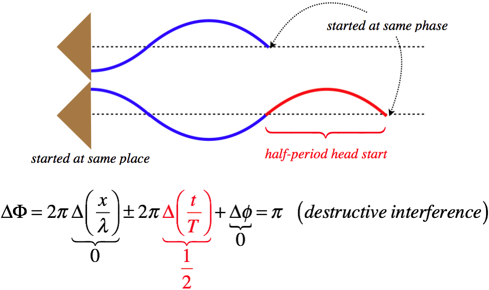
Case 2: Different Time Intervals (\(\Delta x=0\), \(\Delta t\ne 0\), \(\Delta \phi=0\))
Next we will place the speakers side-by-side, so that the travel distances of the waves at any position in the medium is the same. As before, the leading wave front of the waves will be in phase, but this time we will turn on one of the speakers at a time of one-half period before the other speaker. This lag between the two once again throws the two waves out of phase, resulting in destructive interference:
Figure 1.4.4 – Destructive Interference Due to Starting Time Only
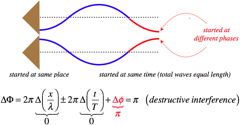
Case 3: Different Starting Phases (\(\Delta x=0\), \(\Delta t=0\), \(\Delta \phi\ne 0\))
Now finally, we will position speakers side-by-side, and turn them on at the same moment, but will arrange things so that the sounds they emanate leave the speakers \(\pi\) radians out of phase, to get the same destructive interference:
Figure 1.4.5 – Destructive Interference Due to Phase Constant Only
One More Case: Different Perspectives
While these all seem distinctly different, very often the same interference effect can be described in any of the three ways, simply by changing our perspective. To see this, let's consider a two-dimensional harmonic wave coming from a single point source. This could be a wave caused by a pebble dropped into a pond, for example. This wave radiates circularly-outward from the source. We of course cannot have interference with only one wave, so we will provide a means to split it into two separate waves: The wave will strike a barrier with two small holes in it, through which the wave can pass. As we will see in a future section, these two holes themselves now act like point sources of two separate waves, with the energy of these waves coming from the original wave. It's these two waves that we will allow to interfere.
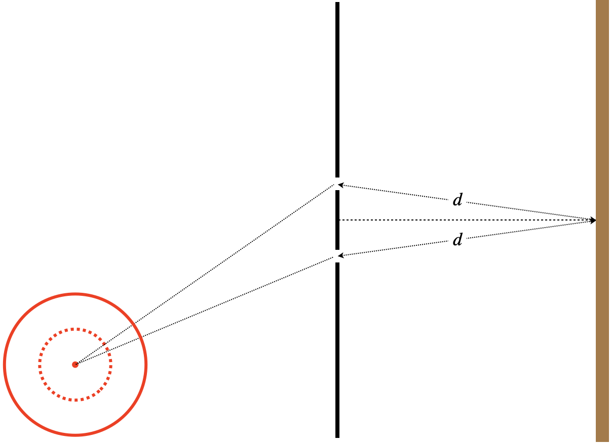
Consider the diagram below. We will be looking at the intensity of the wave when it strikes a second barrier at a position that is equal distances (labeled as '\(d\)' in the diagram) from the two holes. The original source of the wave is not the same distance from both holes, however.
Figure 1.4.6 – Single Source Interference Setup
Suppose we find that the two split waves interfere destructively at the final destination. How can we explain this result? It turns out that we can do it in any of the three ways described above, depending on what perspective we decide to take.
First, we can note that the two waves start at the same time and with the same phase, from the original point source. But these two waves (which initially are part of the same starting wave) do not travel equal distances: \(x_1\ne x_2\). They travel the same distance from the holes to the screen, but the distances to the holes from the starting point are different:
Figure 1.4.7 – Single Source Interference – Distance Traveled Explanation
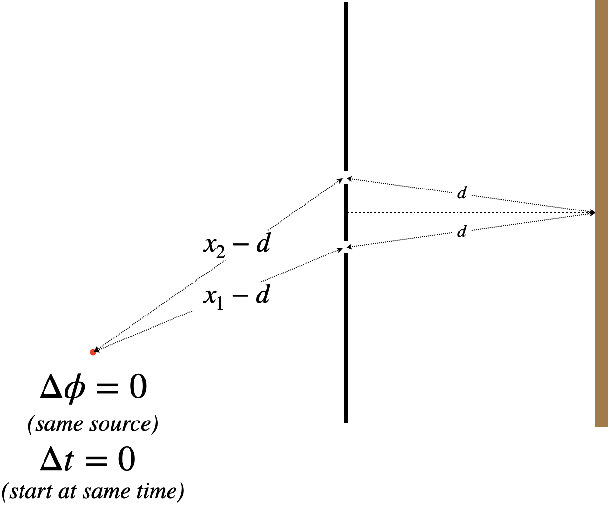
We would see destructive interference if (for example), the extra distance traveled by the wave passing through one hole happens to be a half wavelength farther than the distance traveled by the wave passing through the other hole: \(x_2-x_1=\frac{1}{2}\lambda\).
Now let's change our perspective. Suppose we are watching this wave from the right of the two holes, and know nothing at all about the single point source. As far as we are concerned, the two waves are starting from positions that are the same distance from the position where we are seeing the destructive interference. We would not conclude that the difference in distance traveled is the cause of this interference. But suppose we had been watching since before the first wave emerged from a hole. In this case, we would see a wave with a certain starting phase come out of one hole first, and a short time later, a wave with the same phase come from the other hole. It comes out with the same phase because it comes from the same wavefront from the original point source.
Figure 1.4.8 – Single Source Interference – Time Elapsed Explanation
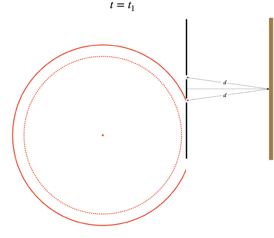
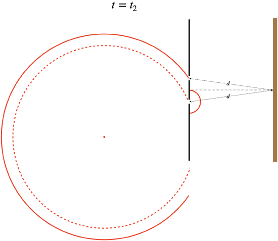
We would see destructive interference if (for example), the time elapsed between when we see the two waves emerge differs by one-half period: \(t_2-t_1=\frac{1}{2}T\).
And finally, there is one other perspective from which we can view this. Once again, we will view the waves from the side of the holes where we can't see the point source, so that we again measure equal travel distances. But this time, let's assume we don't start viewing until after the wave has been passing through both holes for awhile. We look at our watch and note that at time \(t=0\) (when we start watching), there are waves coming from both holes that are out of phase with each other by \(\pi\) radians. Both waves travel the same distance and start at the same time, but start out out of phase, and therefore destructively interfere.
Example \(\PageIndex{2}\)
Two speakers, both pointing in the \(+x\) direction, are placed on the y-axis, separated from each other by a distance of \(2.00\;m\). They emit the same tone, which has a frequency of \(784\;Hz\), in phase with each other. A microphone is placed directly in front of and very close to one of the speakers, and is gradually moved from along the \(x\)-axis farther and farther from the speaker. Assume that the fact that the microphone is a little farther from one speaker than the other does not result in a noticeable intensity difference between the two speakers, so that the sound waves coming from the speakers have the same amplitude when they reach the microphone. The speed of sound waves in air is \(344\frac{m}{s}\).
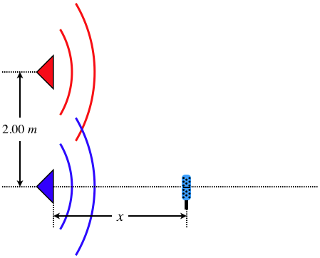
- Find the distances from the closer speaker where the microphone detects no sound.
- Find the distances from the closer speaker where the sound gets loudest (i.e. constructive interference).
- Suppose the tone coming from the speakers has an adjustable frequency, and that it is gradually lowered. Find the frequency below which the microphone has no position on the \(x\)-axis where it measures total silence.
- Solution
-
a. The starting phase and time are the same, so the only source of phase difference comes from the difference in distance traveled. From the \(\Delta x\) contribution to the phase difference that causes destructive interference (i.e. when the extra distance is an odd number of half-wavelengths), we therefore have:
\[\dfrac{2\pi}{\lambda}\Delta x = n\pi \;\;\;\Rightarrow\;\;\; \Delta x = \frac{1}{2}n\lambda\;, \;\;\;\;\;n=1,\;3,\;5,\;\dots \nonumber\]
The difference in distances traveled by the two waves us found using the Pythagorean theorem, so putting this in above gives:
\[\Delta x = \sqrt{x^2+\left(2.00\;m\right)^2} - x = \frac{1}{2}n\lambda \]
Calling the \(n^{th}\) value of \(x\) "\(x_n\)" and doing the algebra gives:
\[x_n=\frac{1}{n\lambda}\left(4.00m^2-0.250n^2\lambda^2\right)\nonumber\]
We are given the frequency of the sound, so we can find its wavelength:
\[\lambda = \frac{v}{f} = \dfrac{344\frac{m}{s}}{784Hz}=0.439m\nonumber\]
Notice that although the value of \(n\) is not restricted, when it gets too high, the value of \(x_n\) will become negative. Plugging in all of the values of \(n\) that give positive values of \(x\) yields five possible values:
\[x_1=9.00m,\;\;\;x_3=2.71m,\;\;\;x_5=1.27m,\;\;\;x_7=0.531m,\;\;\;x_9=0.022m\nonumber\]
b. Constructive interference occurs when the path difference is an even number of half-wavelengths (i.e. some number of full wavelengths). We can get our answer directly from part (a) simply by taking even values of \(n\) instead of odd values. Once again, the number of values of \(n\) is limited by the restriction that sign of \(x_n\) must be positive.
\[x_2=4.34m,\;\;\;x_4=1.84m,\;\;\;x_6=0.858m,\;\;\;x_8=0.259m\nonumber\]
c. The value of \(\Delta x\) clearly gets smaller as \(x\) gets larger (the hypotenuse gets closer and closer to equaling the \(x\) value as \(x\) gets larger), so the largest possible value of \(\Delta x\) is just the separation of the speakers. If the speakers are separated by less than one-half wavelength, then \(\Delta x\) can never get as big as a half wavelength, and no totally destructive interference is possible. These speakers are separated by \(2.00\;m\), so the wavelength of the sound must be shorter than \(4.00m\) for there to be any instance of total destructive interference. This wavelength corresponds to a frequency of:
\[f = \frac{v}{\lambda} = \dfrac{344\frac{m}{s}}{4.00m} = 86Hz \nonumber\]
Frequencies lower than this create wavelengths that are so long that \(\Delta x\) is never large enough to cause total destructive interference.
Video Lecture