
1.3: Energy Transmission


- Last updated
- Nov 8, 2022
- Save as PDF

( \newcommand{\kernel}{\mathrm{null}\,}\)
1-Dimensional Waves
While we will be interested in energy transmission in all kinds of waves, we will start with 1-dimensional harmonic waves as our model, as we are already familiar with the harmonic motion exhibited by the medium as such a wave passes. In particular, we have an idea of how to deal with the energy of a single oscillating particle, so for now we will also restrict ourselves to mechanical waves, where the particle comprising the medium are actually oscillating (i.e. think about a transverse wave on a string).
The energy of a single oscillating particle comes in two forms: kinetic and elastic potential (we'll maintain the convention that the particle is displacing in the y direction as the wave moves in the ±x direction):
Etot=KE+PEelastic=12mv2+12ky2
Of course both the speed of the particle and its displacement are changing with time, so it's more useful to express the energy of this particle in terms of one of the constants of the motion. When the particle reaches its maximum displacement, it stops moving, so its kinetic energy goes to zero and all of the energy is potential. But we have given this maximum displacement a name – amplitude. So the total energy of the oscillating particle is:
One might complain that there are no springs present for this kind of wave, so what are we supposed to plug into k? Well, there is a restoring force on every particle in the string as the wave passes, and this behaves like the restoring force of a spring, but we can write this expression more appropriately if we replace the spring constant with an equivalent expression in terms of the mass of the particle and the frequency of oscillation. Recall that for simple harmonic motion we have:
2πf=ω=√km⇒k=m(2πf)2
Now the energy of the particle is in terms of the medium (the mass of the particle) and the wave (the amplitude and frequency):
We stated at the very beginning that waves carry energy from one point to another. Now that we see that a single particle in the medium carries energy, it should be clear that this is true. Consider a wave pulse that is harmonic for just one wavelength:
Figure 1.3.1 – Wave Pulse Carries Energy
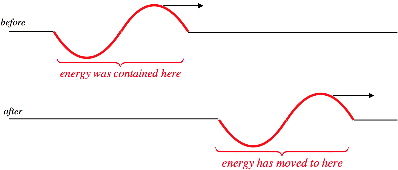
Clearly the region where the particles are oscillating changes in this case, which means that the region that contains the energy is changed. The pulse transports energy across the expanse by having particles in the medium transfer energy to their nearest-neighbors, without the particles themselves having to make the trip.
Suppose we wish to know how much energy is in the whole wave, rather than what is just in a single particle. In this case, we treat the wave as continuous, with an infinite number of infinitesimal particles oscillating. The mass of these particles is very small, and can be written in terms of the mass density of the medium (again, think of this as a wave on a string), multplied by a small segment along the x direction:
dm=μdx
We can now use this mass to express the infinitesimal amount of energy possessed by that particle, by plugging this into Equation 1.3.4:
dE=12dm(2πf)2A2=12μdx(2πf)2A2
This is the energy in a single particle of the medium within the wave, so to get the full energy carried by the wave, we need only add up all these parts by performing an integral. The range of the single wave goes for one wavelength, so choosing the origin to be at one end of the wave, we have:
Einwave=∫inwavedE=λ∫012μdx(2πf)2A2=12μ(2πf)2A2λ∫0dx=12μ(2πf)2A2λ
Of course, if we have a full harmonic wave, as described by the wave function given in Equation 1.2.7, we have an infinite number of these single wave pulses, and the amount of energy in the entire wave is infinite and uninteresting. What is finite, even in the case of a full harmonic wave, is the rate as which energy is being transferred. To compute this, we simply need to divide how much energy a single wave pulse is carrying by the time it takes to completely cross some fixed point. Well, we know that this time interval is one period, so we have for the power of the wave:
Pwave=EonewavepulseT=12μ(2πf)2A2λT=12μ(2πf)2A2v,
where v is the speed of the wave. We can put this entirely in terms of the constants of motion of the wave and the medium for our case of a wave on a string by plugging in for the velocity in terms of the string tension and mass density (Equation 1.2.17):
This calculation is specific to harmonic waves on strings, and we will not go into how this result changes for other types of harmonic waves (which pass through different sorts of media, may not be mechanical in nature, etc.). However, we will note that for a one-dimensional wave, the power is proportional to the square of the amplitude. As we will see, we will need to modify this result slightly for waves in two and three dimensions.
Multi-Dimensional Waves
In Section 1.1 we found that in order to satisfy the wave equation, waves that propagate out from a central source, into two or three dimensions cannot repeat their waveform. Here we will see why that is so, and get some idea of specifically how the waveform changes. Again, we will remain within the confines of our harmonic wave model for simplicity. First we need to clarify an important assumption: In our discussion we will assume that dissipative effects of the medium are negligible. That is, the particles in the medium that oscillate do so without "friction." This means we are assuming that all of the energy in the wave remains within the wave, and none of the energy is converted into thermal energy in the medium.
Consider now a wave radiating outward from a point source in two dimensions (think of a circular ripple on a pond caused by a pebble). Each position in the medium contains a particle oscillating harmonically (like a mass on a spring), and as the wave propagates outward, the number of oscillating particles increases. The particles in the medium are spaced the same everywhere, so the number of particles encountered by the circular wave is proportional to its circumference, and therefore proportional to its radius. This means that when the radius of the wave front doubles, it is oscillating twice as many particles in the medium.
Figure 1.3.2 – Circular Wave Energy Conservation
As the wave moves out, there is no energy lost, so the when the circle enlarges, the energy is distributed amongst a larger number of oscillators. The energy in each oscillator is determined by its amplitude of oscillation, so for more oscillators to have the same energy as fewer oscillators, their amplitudes must decrease. Specifically, the energy per oscillator is proportional to the square of the amplitude (Equation 1.3.2), which means that doubling the radius of the circle reduces the amplitude by a factor of √2, tripling the radius reduces the amplitude by a factor of √3, and so on. The figure above shows what happens to the amplitude of the wave in cross-section as it goes from a radius of 1 wavelength to 3 wavelengths.
The wave doesn't change its velocity from the inner circle to the outer circle, so the rate at which energy passes through each circle must be the same. What is different about two circles is the density of the energy contained in each. For the smaller circle, the energy is distributed over a smaller circumference than for the larger circle, so the energy density becomes smaller as the wave propagates outward. We can define power density in the same manner – by dividing the power of the wave (which is the same for both rings, and everywhere else) by the size of the region through which it is passing. This "power density" is called intensity. For our two-dimensional wave, this is the ratio of the power of the wave and the circumference of the circle through which it is passing:
I2d(r)=P2πr
Therefore the intensity of a two-dimensional wave radiating outward from a central point varies in inverse proportion to the distance from the central source. We find that the intensity is proportional to the square of the amplitude:
A∝1√r⇒I∝A2
It turns out that the proportionality of intensity and square amplitude was the case for one-dimension as well. For a one-dimensional wave, the energy density does not change, because all of the energy is handed from one oscillator to another neighboring single oscillator. Therefore the power density (intensity) doesn't change, which is consistent with what we already know; the amplitude of a one-dimensional wave remains constant.
Far more common in our studies are three-dimensional waves with central sources (namely sound and light), and the power density in these cases involves dividing by a spherical surface area, rather than a circle. In this case, the intensity of the wave has units of watts per square meter (whereas the intensity of the two-dimensional wave had units of watts per meter), and we have:
I3d(r)=P4πr2
Once again we find the same relationship between intensity and amplitude. The same mechanism is at work: As the wave moves outward from a central point, the number of oscillators on each spherical surface is proportional to the surface area. Doubling the radius of a spherical surface quadruples the surface area, so the number of oscillators grows with the square of the radius. This means that the energy per oscillator drops with the square of the radius, and the amplitude is inversely-proportional to the radius:
A∝1r⇒I∝A2
The relation between intensity and amplitude is therefore universal among waves, and one that we will keep in mind in the sections to come.
Note that this intensity drops faster than that of the two-dimensional wave, satisfying what's known as an inverse-square law: The intensity gets weaker in inverse proportion to the square of the distance from the source. Since the power of the wave is the same everywhere, we have the following relationship of intensities at two distances r1 and r2 from the source for waves that propagate outward from a point source:
Digression: Return to the Wave Equation
We can look to the wave equation in two and three dimensions to see if the relationship we obtain above between amplitude and radius actually holds true. For subtle reasons that we won't go into, it does hold true for three dimensions, but is only approximately true for two dimensions (the approximation improves as the wave gets farther from the source). If we accept the two-dimensional approximation, then we have a nice extension of the description of the wave function we gave in Section 1.1:
1dimension:f(x,t)=f(x±vt)2dimensions:f(r,t)=f(r±vt)√r(approximate,forlarger)3dimensions:f(r,t)=f(r±vt)r
To demonstrate these relations, one must write the wave equation in polar coordinates for two and three dimensions, respectively. For the reader that may be inspired to give demonstrating this a try, here are the double spatial derivatives for each case:
2dimensions:∇2f=1r∂∂r(r∂f∂r)3dimensions:∇2f=1r2∂∂r(r2∂f∂r)
Example 1.3.1
At time t=0, a plunger begins oscillating up-and-down at a steady rate for 6 full oscillations in a body of otherwise calm water. During this time, it puts 420J of energy into the surface waves it creates. The wavelength of the wave is measured to be 1.0m, and the wave speed is measured to be 1.2m/s.

- Find the power supplied by the plunger.
- Find the intensity of the leading wavefront at time t=4.0s.
- The amplitude of the leading wavefront at t=4.0s is measured to be 5.4cm. Find its amplitude at t=8.0s.
- Solution
-
a. The power is the rate at which the energy is being transferred into the waves. We know how much energy is put into 6 oscillations, so if we divide that energy by the time span of 6 oscillations, we have the value of the power. The time span of 6 oscillations is 6 periods, and a single period we can calculate from the wavelength and wave speed:
T=λv=56s⇒Δt=6T=5.0s⇒P=EΔt=420J5s=84W
b. To get the intensity, we need to know the circumference of the leading wavefront. We know the speed of the wave and how long it has been traveling, so:
r=vΔt=(1.2ms)(4.0s)=4.8m⇒I=P2πr=84W2π4.8m=2.8Wm
c. For the two-dimensional wave, the amplitude gets smaller as the radius grows, by a factor of 1√r. The wave's speed is unchanging, so after 8 seconds the wave has traveled twice as far from the source than after 4 seconds. Doubling the distance traveled therefore reduces the amplitude by a factor of √2, giving:
A(t=8.0s)=A(t=4.0s)√2=5.4cm√2=3.8cm