6.1: Linking Linear and Angular Momentum

Rotational Impulse-Momentum Theorem

By now we have a very good sense of how to develop the formalism for rotational motion in parallel with what we already know about linear motion. We turn now to momentum. Replacing the mass with rotational inertia and the linear velocity with angular velocity, we get:

\[ \overrightarrow p \equiv m \overrightarrow v \;\;\; \iff \;\;\; \overrightarrow L \equiv I \overrightarrow \omega \]

The vector \(L\) is called angular momentum, and it has units of:

\( \left[ L \right] = \dfrac{kg \cdot m^2}{s} = J \cdot s \)

Continuing the parallel with the linear case, the momentum is relates to the force through the impulse-momentum theorem, which is:

\[ \int \limits_{t_A}^{t_B} \overrightarrow F_{net} dt = \Delta \overrightarrow p_{cm} \;\;\; \iff \;\;\; \int \limits_{t_A}^{t_B} \overrightarrow \tau_{net} dt = \Delta \overrightarrow L \]

While there is no need to append "cm" to the angular momentum as we do with the linear momentum, we do have to keep in mind that all of the quantities in the rotational case must be referenced to the same point. That is, the net torque requires a reference point, and the angular momentum contains a rotational inertia, which also requires a reference point.

Recall that the impulse-momentum theorem is just a repackaging of Newton's second law, and so it is with the rotational case, though there is a twist, as we will see shortly:

\[ \overrightarrow F_{net} = \dfrac{d\overrightarrow p_{cm} }{dt} = \dfrac{d\left(m\overrightarrow v_{cm}\right) }{dt} = m\overrightarrow a_{cm} \;\;\; \iff \;\;\; \overrightarrow \tau_{net} = \dfrac{d \overrightarrow L}{dt} = \dfrac{d\left(I\overrightarrow \omega\right) }{dt} = I\overrightarrow \alpha \]

Analyze This

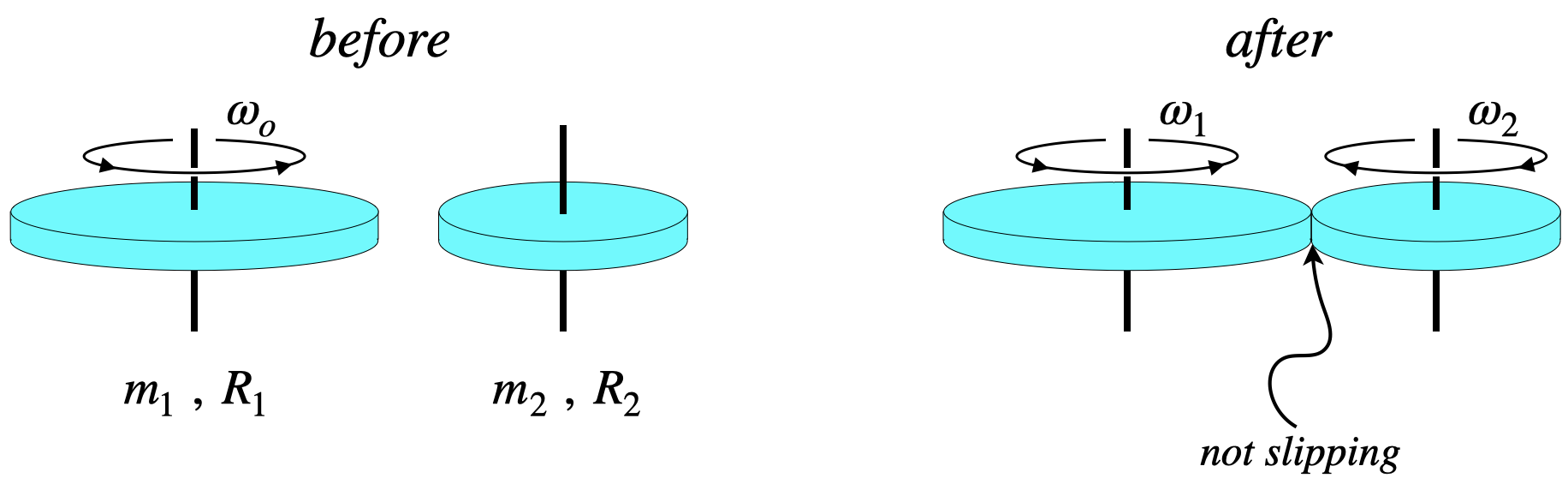
Two uniform disks are free to rotate frictionlessly around vertical axles. Initially one of the disks is rotating, while the other is not.  They are then brought together so that their outer edges rub against each other. Kinetic friction between the two rubbing surfaces slows down disk #1, while speeding up disk #2.  This continues until their rotational speeds are such that no slipping occurs between the two surfaces. With kinetic friction no longer present, they continue with constant rotational motion from this point forward.

Analysis

The surfaces stop slipping when the outer edges of the two disks are moving at the same linear (tangential) speed. We therefore have the "after" constraint:

\[v_1=v_2~~\Rightarrow~~R_1\omega_1=R_2\omega_2\nonumber\]

The friction force exerts torques on both disks. Newton's 3rd law ensures that each disk experiences the same magnitude of kinetic friction, and for the same period of time, but the torques about their axles are different, because the moment-arms are not equal (the disks have different radii). So the two disks experience different magnitudes of rotational impulse, and the ratio of the magnitudes of these impulses is:

\[\dfrac{\left|\tau_1\right|\Delta t}{\left|\tau_2\right|\Delta t}=\dfrac{f_kR_1\Delta t}{f_kR_2\Delta t}=\frac{R_1}{R_2}\nonumber\]

These rotational impulses equal the changes in the angular momenta of their respective disks, which we can write in terms of the before & after values:

\[\left|\Delta L_1\right|=I_1\left|\Delta\omega_1\right|=\frac{1}{2}m_1R_1^2\left(\omega_o-\omega_1\right)\nonumber\]

\[\left|\Delta L_2\right|=I_2\left|\Delta\omega_2\right|=\frac{1}{2}m_2R_2^2\left(\omega_2-0\right)\nonumber\]

Plugging these angular momentum changes into the impulse ratios above gives:

\[\dfrac{\left|\Delta L_1\right|}{\left|\Delta L_2\right|}=\dfrac{\left|\tau_1\right|\Delta t}{\left|\tau_2\right|\Delta t}~~\Rightarrow~~\frac{m_1}{m_2}\frac{R_1^2}{R_2^2}\left(\dfrac{\omega_o-\omega_1}{\omega_2}\right)=\frac{R_1}{R_2}~~\Rightarrow~~\frac{m_1}{m_2}\left(\dfrac{\omega_o-\omega_1}{\omega_2}\right)=\frac{R_2}{R_1}\nonumber\]

We can now use our constraint on the two "after" angular speeds to solve for each of them:

\[\frac{m_1}{m_2}\left(\dfrac{\omega_o-\omega_1}{\frac{R_1}{R_2}\omega_1}\right)=\frac{R_2}{R_1}~~\Rightarrow~~\omega_1=\left(\dfrac{m_1}{m_1+m_2}\right)\omega_o\nonumber\]

\[\omega_2=\frac{R_1}{R_2}\omega_1~~\Rightarrow~~\omega_2=\frac{R_1}{R_2}\left(\dfrac{m_1}{m_1+m_2}\right)\omega_o\nonumber\]

Link Between Angular and Linear Momentum

When there are several particles in a system, we find the momentum of the system by adding the momenta of the particles:

\[ \overrightarrow p_{cm} = \overrightarrow {p_1 }+ \overrightarrow {p_2} + \dots \]

We have a definition for the angular momentum of a rigid object, but can we define the angular momentum of a single particle, and then add up all of the angular momenta of the particles to get the angular momentum of the system, in the same way that we do it for linear momentum? The answer is yes, but we have to be careful about our reference point. That is, to add the angular momentum of every particle together to get a total angular momentum, the individual angular momenta must be measured around the same reference.

So how do we define the angular momentum of an individual particle around a certain reference point? Let's look at a picture of the situation. The particle has a mass \(m\), a velocity \(\overrightarrow v\), and is located at a position \(\overrightarrow r\) with the tail of that position vector at the reference point.

Figure 6.1.1a – Angular Momentum of a Point Particle

If this particle was a part of a rigid body rotating around the reference point, the parallel component of the velocity vector would be zero. So it makes sense to exclude that part of the velocity vector when defining the angular momentum of this particle. We know the rotational inertia of the point particle, and the relation between \(v_{\bot}\) and \(\omega\), so we get for the magnitude of the angular momentum:

\[ L_{single\;particle} = I \omega = \left[mr^2\right] \left[\dfrac{v_{\bot}}{r}\right] = mrv_{\bot} = mrv\sin\theta \]

Suppose the particle continues moving free of any forces. What happens to its angular momentum? Let's look at what happens to the picture:

Figure 6.1.1b – Angular Momentum of a Point Particle

What a mess! The mass and velocity vector remain the same, but everything else changes. How can we determine what happens to the angular momentum? Well, have a look at Equation 6.1.2. With no force on the particle, there can't be any torque on the system, so the angular momentum must remain unchanged. It turns out there is a simpler way to look at the angular momentum, to see why this must be the case.

Figure 6.1.1c – Angular Momentum of a Point Particle

We can define the quantity \(r_{\bot}\) in a manner similar to how we defined moment arm – it is the perpendicular distance from the reference point to the line along which the particle is moving. Doing this gives us an alternative way of writing the magnitude of the particle's angular momentum. Using the fact that \(r_{\bot}=r\sin\theta\), we have:

\[ L_{single\;particle} = mrv_{\bot} = mrv\sin\theta = mvr_{\bot} \]

Now it is quite easy to see that the angular momentum of the particle doesn't change while it moves – it keeps the same mass and speed, and stays on the same line, so \(r_{\bot}\) doesn't change either.

Angular momentum is a vector, so what direction does it have here? Going back to the idea of this particle being part of a rigid object, it's clear that this object would be rotating clockwise around the reference, so from the right hand rule, the vector must point into the page. We would like a mathematical expression of this, and as with the case of torque, it comes from the cross product. The two vectors involved are the position vector and the velocity vector, and indeed we see that the following cross product results in the correct direction, and takes care of the \(\sin\theta\) contribution as well:

\[ \overrightarrow L_{single\;particle} = m\overrightarrow r \times \overrightarrow v = \overrightarrow r \times \overrightarrow p \]

This is a nice, compact expression of the relation between the linear momentum of a particle and its angular momentum around a reference point. To see this relation come full circle, imagine that a force is exerted on the particle. This would cause the momentum to change. It would also result in a torque on the system about the reference point, causing the angular momentum to change. Taking the derivative of Equation 6.1.7 with respect to time gives:

\[ \overrightarrow \tau = \dfrac{d\overrightarrow L}{dt} = \dfrac{d}{dt}\left(\overrightarrow r \times \overrightarrow p\right) = \dfrac{d\overrightarrow r}{dt} \times \overrightarrow p + \overrightarrow r \times \dfrac{d\overrightarrow p}{dt} = \overrightarrow v \times \overrightarrow p + \overrightarrow r \times \overrightarrow F \]

The velocity vector is parallel to the momentum vector, so the cross product in the first term is zero, leaving us with a relation between torque and force that we have seen before (Equation 5.4.6).

Now that we can deal with the angular momentum of a single particle relative to some reference point, we can simply add the contributions of many such particles within a system, relative to the same reference point:

\[ \overrightarrow L_{system} = \overrightarrow r_1 \times \overrightarrow p_1 + \overrightarrow r_2 \times \overrightarrow p_2 + \dots \]

Note that these particles may be part of a rigid object, or may not be bound to each other at all. If they happen to be bound into a single rigid object rotating around a fixed point on the object, then the result is more easily expressed in terms of the rigid object's rotational inertia and angular velocity (Equation 6.1.1):

\[\begin{array}{l} \overrightarrow L_{rigid\;object} && = && \overrightarrow r_1 \times m_1\overrightarrow v_1 + \overrightarrow r_2 \times m_2\overrightarrow v_2 + \dots \\ && = && \left[r_1\widehat r_1\right] \times m_1\left[v_1\widehat v_1\right] + \left[r_2\widehat r_2\right] \times m_2\left[v_2\widehat v_2\right] + \dots \\ && = && \left[r_1\widehat r_1\right] \times m_1\left[r_1\omega\widehat v_1\right] + \left[r_2\widehat r_2\right] \times m_2\left[r_2\omega\widehat v_2\right] + \dots \\ && = && m_1 r_1^2\left[\omega\widehat r_1 \times \widehat v_1\right] + m_2 r_2^2\left[\omega\widehat r_2 \times \widehat v_2\right] + \dots \\ && = && m_1 r_1^2\left[\omega\widehat \omega\right] + m_2 r_2^2\left[\omega\widehat \omega\right] + \dots \\ && = && I\overrightarrow\omega \end{array}\]

Consider next an extended object that is not rotating, but is moving in a straight line relative to some reference point. Despite the fact that it is not rotating, it can have angular momentum relative to that reference point. Writing the angular momentum of the whole object as a sum of the angular momenta of its particles, we get:

\[ \overrightarrow L_{not-rotating\:extended\:object} = m_1\overrightarrow r_1 \times \overrightarrow v_1 + m_2\overrightarrow r_2 \times \overrightarrow v_2 + \dots \]

With the object not rotating and all the particles held rigidly in place, every particle has the same velocity, which equals the velocity of the object's center of mass, so this can be factored out of all the cross products, giving:

\[ \overrightarrow L_{not-rotating\:extended\:object} = \left(m_1\overrightarrow r_1 + m_2\overrightarrow r_2 + \dots\right) \times \overrightarrow v_{cm} = \left(\dfrac{m_1\overrightarrow r_1 + m_2\overrightarrow r_2 + \dots}{M}\right) \times \left(M\overrightarrow v_{cm}\right) = \overrightarrow r_{cm} \times \overrightarrow p_{cm} \]

What this means is that an extended object moving in a straight line has the same angular momentum relative to a reference point as a point particle located at the object's center of mass, with the same mass and velocity.

If the extended object has both its center of mass moving at a constant velocity relative to the reference point and it is also rotating around an axis through its own center of mass, then things get complicated. We won't into the details of the most general case, but it is not unreasonable to consider the case of the linear velocity lying in the plane perpendicular to the rotation vector (e.g. an object moving within this screen while rotating around an axis perpendicular to this screen – see Figure 6.1.2).

Figure 6.1.2 – Total Angular Momentum

The total angular momentum comes out to be reminiscent of the parallel-axis theorem and of the kinetic energy being the sum of linear and rotational parts:

\[ \overrightarrow L_{tot} = \overrightarrow L_{rotation\; around \:cm} + \overrightarrow L_{cm \; moving \; by\;reference \; point} = I_{cm} \overrightarrow \omega + \overrightarrow r_{cm} \times \overrightarrow p_{cm} \]

An interesting and important consequence of this is that an object that is only rotating around its center of mass (but not moving linearly) has the same angular momentum measured relative to every reference point.

Analyze This

The center of a uniform solid disk is threaded onto an axle at the end of a thin uniform rod. The rod and the disk have equal masses, and the radius of the disk is one-third the length of the rod. The rod is attached to a fixed pivot point at its other end, around which it is free to rotate. With the rod and disk both starting from rest, a force of constant magnitude is exerted tangent to the edge of the disk at the point farthest from the pivot for a short time. There is no gravity present.

Analysis

We'll start by creating a couple of labels. The mass of the disk and the rod are the same, and we will call this mass \(m\). The radius of the disk we will call \(R\), and the rod is three times this long, so its length is \(3R\).

The disk + rod system is given a rotational impulse about the pivot point, so its angular momentum will change. The force exerted is a distance \(4R\) from the pivot, and is directed perpendicular to the line joining the pivot and the point where it acts, so it delivers a total torque of \(\tau=4RF\). Multiplying this constant torque by the time span over which it acts gives the total impulse, and therefore the total angular momentum of the system.

This angular momentum is manifested in three ways: 1. The disk rotates around its center, 2. The disk moves in a circular path around the pivoted end of the rod, 3. The rod rotates around its pivoted end. The rotational speeds for the last two cases are the same, and we'll call this speed \(\omega_1\). The rotational speed of the disk about its center we'll call \(\omega_2\). With these definitions in place, the magnitude of the angular momentum of the system about the fixed pivot is:

\[L_{system} = L_{disk}+L_{rod} = \left(I_{disk}\omega_2+mr^2\omega_1\right)+I_{rod}\omega_1\nonumber\]

Plugging-in \(r=3R\) (the center of mass of the disk is one rod-length from the pivot) and the moments of inertia of the rod and disk, we get:

\[L_{system} =\frac{1}{2}mR^2\omega_2+m\left(3R\right)^2\omega_1+\frac{1}{3}m\left(3R\right)^2\omega_1=mR^2\left(12\omega_1+\frac{1}{2}\omega_2\right)\nonumber\]

We know this equals the impulse delivered by the torque, but the problem is well-specified, so we should be able to to do more than write the answer in terms of two angular speeds – they should be related to each other somehow. To work this out, we have to deal with the disk and rod as separate systems. A couple of free-body diagrams are therefore called-for:

A quick explanation of these FBDs: \(N\) is the normal force by the axle on the disk, reacting to the applied force \(F\). \(T\) is the "tension" force keeping the disk moving in a circle. \(V\) is the vertical force by the pivot that makes sure there is a net force which keeps the center of mass of the rod moving in a circle. Neither \(T\) nor \(V\) contribute to any torques. We'll say that \(F\) and \(N\) act for a time \(\Delta t\) to contribute to their respective rotational impulses.

The net torque on the rod about the pivot is \(3RN\). Multiply this by the time it acts (and remembering that it starts from rest), we have, from the impulse-momentum theorem:

\[3RN\Delta t = I_{rod}\omega_1 = \frac{1}{3}m\left(3R\right)^2 \omega_1 \;\;\; \Rightarrow \;\;\; N\Delta t = mR\omega_1\nonumber \]

The net torque on the disk about its center is \(FR\), so:

\[ FR\Delta t = I_{disk}\omega_2 = \frac{1}{2}mR^2 \omega_2 \;\;\; \Rightarrow \;\;\; F\Delta t = \frac{1}{2}mR \omega_2 \nonumber \]

[Note: While it might appear as though this rotational impulse determines the rotational motion of the disk relative to the rod, it does not. The resulting motion is the total angular velocity (relative to the lab). If this force was zero, and the rod is made to turn without any torque on the disk (i.e. the force is applied to the rod instead of the disk), the disk would maintain its orientation relative to the lab as the rod rotates, turning relative to the rod in the opposite direction at the same rate that the rod rotates. In this case, \(\omega_2\) would be zero, which matches the zero value of \(F\).]

We need one more equation, and it comes from the linear impulse-momentum theorem for the disk. From the FBD, we see that the net force on the disk is \(F-N\), and this results in a change of (tangential) momentum of \(mv_{cm}\). The final linear velocity of the disk's center of mass is directly related to \(\omega_1\) (it moves with the end of the rod) so:

\[\left(F-N\right)\Delta t = mv_{cm} = m\left(3R\omega_1\right) \nonumber \]

Putting these last three equations together gives a relationship between \(\omega_1\) and \(\omega_2\):

\[ \frac{1}{2}mR \omega_2 - mR\omega_1 = 3mR\omega_1 \;\;\; \Rightarrow \;\;\; \omega_2 = 8\omega_1 \nonumber \]

This can be put back into the equation for the system's total angular momentum to get:

\[L_{system} =16mR^2\omega_1=2mR^2\omega_2\nonumber\]