
1.16: Parallax, Cepheid Variables, Supernovae, and Distance Measurement


- Last updated
- Feb 23, 2025
- Save as PDF

( \newcommand{\kernel}{\mathrm{null}\,}\)
We have seen from the previous chapters, at least on very large scales, the Universe is the same everywhere and that it is expanding. Key to observing the consequences of this expansion is the ability to measure distances to things that are very far away. Here we cover the basics of how that is done. We have to do it in steps, getting distances to nearby objects and then using those objects to calibrate other objects that can be used to get to even further distances. We refer to this sequence of distance determinations as the distance ladder.
The first rung on this ladder is the use of trigonometric parallax to determine distances to the nearest stars. Some of these nearest stars are Cepheid variable stars with a luminosity that varies over time in a periodic manner. These stars have a relationship between the period of their luminosity variation and average lumniosity. With distances determined to some of them, that relationship can be calibrated. Once calibrated, then by determining their period, we can determine their luminosity and use them as standard candles to measure even further distances. Cepheids, in turn, can be used to calibrate type Ia supernova explosions. Supernovae are much much brighter than Cepheids, allowing us to observe them to even greater distances.
There's a very good and entertaining 3Blue1Brown YouTube video about the distance ladder you might want to check out. The video covers parallax and Cepheid variable stars, providing more information about these steps in the distance ladder than we manage to include here, and with some pretty cool animations. It also covers an earlier rung in the distance ladder we entirely neglect here: how to determine the Earth-Sun distance. Unfortunately it neglects supernovae, and treats redshift measurements as if they are a means to get a distance measurement -- which they are if you assume a specific cosmological model. This is a different perspective from our own, since we want to use measurements of distance and redshift to determine cosmological model parameters. Thanks to UC Davis student Peyton Harris for pointing this video out to me.
Direct observations - Parallax
Parallax is the shift in apparent location of a nearby object relative to more distant objects, as one changes the observation point. The phenomenon can readily be observed by holding your thumb out in front of you and switching your viewpoint from left eye to right eye and back. Simple trigonometry, and the small-angle approximation, lead to the relationship d=baseline/p where p is the "parallax angle" in radians, and the baseline is half the distance between your two eyes.
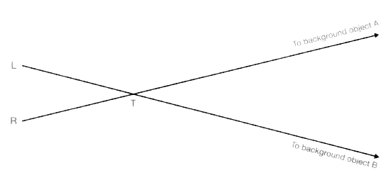
The drawing below in the astronomical context has the parallax angle labeled on an angle with vertex at the nearby star. This is NOT actually the angle that gets directly measured, but rather is geometrically inferred from an angle that is measured.
Box 1.16.1
Exercise 16.1.0: In the figure below, L is left eye, R is right eye, and T is thumb held out at arm's length. Assume that the background objects that line up with the eyes and the thumb (both A and B) are effectively infinitely far away. i) Draw the angle (by adding it to the figure below) that one can actually observe with your right eye. Note: you will need to add the line from R to background object B in order to indicate this angle. ii) Draw in the baseline as described above, b. iii) Using the small-angle approximation and assuming the measured angle is in radians, relate the thumb-face distance to b and the observed angle you indicated in part i.
Exercise 16.1.1: Use observations of trigonometric parallax to estimate the length of your arm in units of your inter-ocular distance (IOD). That is, how many times longer is your arm than the space between your eyes. Since you don’t have a protractor on you to measure angles, I’ll tell you that your thumb, at the joint closer to the tip, held at arm’s length subtends an angle of about 2 degrees. What is, roughly, the distance between your eyes in cm? Does the result you get for the length of your arm make sense?
The change in a star's position in the sky as a result of its true motion through space is called proper motion. This is distinguished from the annual apparent motion in the sky caused by the Earth's orbit around the Sun. A nearby star's apparent movement against the background of more distant stars is referred to as stellar parallax.

Box 1.16.2
 |
| These images of the sky toward star cluster Knox0325 were taken exactly 6 months apart. Each dot is a star. The scale of angular separations is indicated by the line segment toward the bottom of the image which has a length of 0.03 arcseconds. |
Exercise 16.2.1: Use trigonometric parallax to estimate the distance to star cluster KNOX0325 in units of the Earth-Sun distance, known as an astronomical unit or AU. There are 60 arc seconds in an arc minute and 60 arc minutes in one degree.
Exercise 16.2.2: One AU is equal to 1.5×10^13 cm. How far away is KNOX0325 in cm? How far away is it in light years? A light year is the distance light travels in a year and the speed of light is 3×10^10 cm/sec.
Look back at the exaggerated stellar parallax image. The distance to the star is inversely proportional to the parallax. The distance to the star in parsecs is given by
d=1p,
where p is in arc seconds.
The nearest star is proxima centauri, which exhibits a parallax of 0.762 arc sec, and therefore is 1.31 parsecs away.
Box 1.16.3
Exercise 16.3.1: The "parallax angle", p, is defined in such a way that the observed angular shift is equal to 2p. A "parsec" is defined so that one parsec is the distance to an object with p=1 arc sec. How many parsecs away is KNOX0325? The parsec (and kiloparsec, megaparsec and even gigaparsec) is a common unit of measure in cosmology. These are often abbreviated as pc, kpc, Mpc, Gpc.
The limit of measurement from telescopes on the Earth's surface is about 20 parsecs, which only includes nearly 2000 of our closest stars. However, the distance at which parallax can be reliably measured has now been greatly extended by space-based instruments like the Hipparcos satellite and more recently the Gaia satellite.
Box 1.16.4
Exercise 16.4.1: The smallest angular separations that can be measured on the sky, so far, are 0.001 arc seconds (2025 update: about 10 times smaller now). To what distance can parallax be used for determining distances? You can give your answer in parsecs.
While parallax is used to calibrate the cosmic distance scale by allowing us to work out the distances to nearby stars, other methods must be used for much more distant objects, since their parallax angle is too small to measure accurately.
Standard Candles
While stellar parallax can only be used to measure distances to stars within hundreds of parsecs, Cepheid variable stars and supernovae can be used to measure larger distances such as the distances between galaxies and even galaxy clusters. Cepheid variable stars are intrinsic variables which pulsate in a predictable way. In addition, a Cepheid star's period (how often it pulsates) is directly related to its luminosity. The Hipparcos satellite mentioned earlier helped calibrate Cepheid distance scales by measuring the parallaxes of galactic Cepheids.
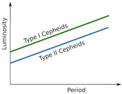
Cepheid variables are extremely luminous and very distant ones can be observed and measured. Once the period of a distant Cepheid has been measured, its luminosity can be determined from the known behavior of Cepheid variables. Then its absolute magnitude and apparent magnitude can be related by the distance modulus equation, and its distance can be determined.
d=10(m−M+5)/5
- d is the luminosity distance to the object in parsecs
- m is the apparent magnitude of the object
- M is the absolute magnitude of the object
Box 1.16.5
Exercise 16.5.1: There is a Cepheid in Galaxy A with a period of 30 days and an apparent magnitude of m=26. How far away is Galaxy A? Use the fact that the Cepheid period-luminosity relation says that a Cepheid with a period of 30 days has an absolute magnitude of M=11. (Note: the answer is 10kpc which is still within our own galaxy so it does not make any sense. I need to update this with a larger apparent magnitude so that it will be further away. If I made it m=36 that would make it 100 times further, which would make it 1Mpc which makes sense. I would then also need to update m for the supernova in Galaxy A (see next Exercise)).
Cepheid variables can be used to measure distances from about 1 kpc to 50 Mpc. Beyond 50 Mpc it becomes too difficult to separate out the light that is just from a Cepheid, from the light from nearby stars. Astronomers call this problem "crowding."
Type Ia supernovae are all caused by exploding white dwarfs which have companion stars. The gravitational pull of the white dwarf causes it to take matter from its companion star. Eventually it reaches a high enough mass that it cannot support itself against gravitational collapse and explodes. All type Ia supernovae reach nearly the same brightness at the peak of their outburst. They then follow a distinct curve as they decrease in brightness. So when astronomers observe a type Ia supernova, they can measure its apparent magnitude at peak brightness. If they know the distance to the supernova, perhaps becaues they have determined using Cepheids the distance to the galaxy hosting the supernova, they can then determine the absolute magnitude of the supernova. We refer to this as supernova calibration. Now, if another supernova is observed, assuming it has the same peak brightness absolute magnitude, we can use measurement of its apparent magnitude at peak brightness to determine its distance.
Box 1.16.6
Exercise 16.6.1: There was also a supernova explosion in Galaxy A (from the previous problem) whose brightness varied with time, but at peak brightness had an apparent magnitude of m=−4.3. What is the absolute magnitude of the supernova at peak brightness?
Exercise 16.6.2: Another supernova went off in Galaxy B and had an apparent magnitude at peak brightness of m=15.7. Assuming supernovae peak brightnesses are standard candles, how far away is Galaxy B?
Type Ia supernovae can be distinguished from other supernovae because they do not have hydrogen lines in their spectra and have a strong Si II line at 615 nm. The peak of their outburst has an absolute magnitude of -19.3±0.03.Type Ia supernovae can be used to measure distances from about 1 Mpc to over 1000 Mpc.
A Standard Ruler
If you observe an object of known length, and determine the angle it subtends, then you can determine the angular diameter distance to the object. As described in the previous chapter, if x is the comoving length of the object and θ is the angle it subtends when oriented so that length runs perpendicular to the line of sight, then the comoving angular diameter distance is, in the small-angle approximation, DA=x/θ. In the previous chapter we also saw that DA=dL/(1+z) where dL is the luminosity distance.
A very important standard ruler in cosmology is the sound horizon. The sound horizon is the distance that a sound wave can travel through the plasma of the big bang, from the beginning until the plasma disappears. We usually denote the comoving sound horizon as rs. Assuming the standard cosmological model, an estimate of the comoving sound horizon given data from the Planck satellite is rs=147.09±0.26 Mpc. The sound horizon leaves an imprint in the matter distribution. We can observe galaxies near some redshift z and measure the statistical properties of both their angular distribution and their distribution with redshift. From this we can infer how the sound horizon projects into an angle perpendicular to the line of sight, θs and how it projects into a redshift separation along the line of sight, δzs. We thus get both a distance estimate: DA=rs/θs and an estimate of H(z) since it turns out that rs=δzs/H(z).
We can calculate rs if we know the sound speed cs and the expansion rate, H(a), and the scale factor when the plasma disappears, ad. In time dt the sound wave travels a comoving distance (physical distance divided by scale factor) of csdt/a(t) so
rs=∫ad0dacs(a)a2H(a).


HOMEWORK Problems
These are all to be done with a computer, except for the first one.
Problem 1.16.1
In the problem following this one you are going to want to have error bars for the distance measurements. But the measurements are actually reported as apparent magnitudes. So you will need to propagate magnitude errors to distance errors. Because a small change in distance, δDA is related to a small change in apparent magnitude δm by δDA=(∂DA/∂m)δm, you can write σ2(DA)=(∂DA/∂m)2σ2(m). Show that, as a result, σ(DA)/DA=0.2ln(10)σ(m)..
Problem 1.16.2
Plot up DA(z) vs. z for the supernova data assuming M=−19.3 which is about what the Cepheid calibration of supernovae give for their absolute magnitude at (corrected) peak brightness. Include error bars in your plot. Label the axes appropriately.
Problem 1.16.3
Calculate DA(z) vs. z for 4 theoretical models. The four cases to include are i) \boldsymbol{H_0 = 73\} km/sec/Mpc; Ωm=0.3,ΩΛ=0.7,Ωk=0, ii) \boldsymbol{H_0 = 67\} km/sec/Mpc; Ωm=0.3,ΩΛ=0.7,Ωk=0, iii) \boldsymbol{H_0 = 73\} km/sec/Mpc; Ωm=1,ΩΛ=0,Ωk=0, iv) \boldsymbol{H_0 = 73\} km/sec/Mpc; Ωm=0.3,ΩΛ=0,Ωk=0.7. Plot up the DA(z) curves with two different z ranges: i) enough to cover all the data and ii) over the interval 0 to 0.2. For both of these choose an appropriate y axis range. Include the data, with error bars, from 16.2 in your plots. This should just be 2 plots.
Problem 1.16.4
Answer these questions based on the graphs in the above problem. Is the z < 0.2 redshift interval relatively insensitive to the density parameters? What parameter is this lower-redshift data sensitive to? Over the whole redshift range, which model would you say provides the best fit to the data? Of the two Hubble constants given, which provides a better fit to the data?
Problem 1.16.5
We use the statistical quantity χ2 as a measure of the quality of agreement of a model prediction with the data. Usually, the lower χ2, the better the agreement. Assuming M=−19.3, calculate χ2 for the 4 above models where
χ2=Σi(mdi−mmi)2/σ2i
with mdi the measured apparent magnitude of the ith supernova (with 'd' for 'data'), mmi is the apparent magnitude of the ith supernva as predicted by the model, and σi is the error on the ith magnitude measurement.