
6.1: More Processes


- Last updated
- Nov 8, 2022
- Save as PDF

( \newcommand{\kernel}{\mathrm{null}\,}\)
Real Processes
We have assumed throughout the previous section that these processes occur quasi-statically. But in real world processes, this is virtually never the case, so one could reasonably wonder what good all of this is. That is, to what extent can we apply results found here to the real world? The answer lies in the idea of the thermodynamic state.
Consider a system in a thermodynamic equilibrium state, which then goes through a real-world (not quasi-static) process, and finally comes back to equilibrium in a different thermodynamic state. It is important to remember that the beginning and ending states are perfectly defined, even if the journey that the system took to get from one to the other is not. This means that changes in state variables from the starting state to the ending state are knowable, because their values are defined at both endpoints. Our knowledge of these special processes provides us with a very useful trick for finding these state variable changes. Let's look at a very simple example.
Example 1 – Computing Volume Change of an Ideal Gas After a Non-Quasi-Static Process
A piston confines n moles of an ideal gas at a pressure P, and is held in place with a constant force. The gas is heated quickly with a flame, and the gas expands non-quasi-statically to a new volume, where a short time later the gas comes back to equilibrium. The force on the piston is the same before and after the expansion, and the starting and ending temperatures are T1 and T2, respectively. Find the change in volume of the gas.
We don't need any "tricks" to solve this, because we have the ideal gas equation of state, which we know applies to the starting and ending equilibrium states. The equal force on the piston before and after means that the starting and ending pressures are equal to P, so we can easily find the change in volume:
PV1=nRT1PV2=nRT2}⇒V2−V1=nRP(T2−T1)
Suppose now that we didn't have this direct route to an answer available to us. A PT process diagram of this situation gives us an idea of what we are up against:
Figure 5.8.7 – A Non-Quasi-Static Process with Equal Starting and Ending Pressures
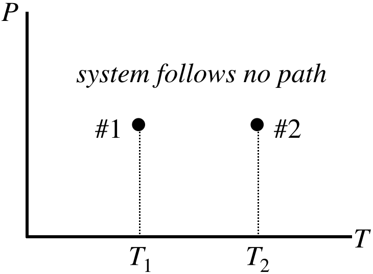
What are we supposed to do with this? Okay, so here is the trick:
Invent any quasi-static process whatsoever that connects the endpoints and use it to compute the change in the state variable.
The value of every state variable at the endpoints is well-defined, so if you can compute these values with a specific process, it doesn't matter if that process didn't actually occur, the resulting values will be correct! Notice that we cannot draw a conclusion about the amount of work done or the amount of heat transferred – these are dependent upon a path through equilibrium states, so picking a path arbitrarily doesn't help with those quantities.
What makes this trick so powerful is that we can often find a very simple quasi-static process to work with. In this particular case, the fact that the starting and ending pressures are equal inspires us to select an isobaric process:
Figure 5.8.8 – Choose an Isobaric Process for the Given Endpoints

Consider the work done over this path. We already solved this for an ideal gas – it can be expressed in two ways: Equation 5.8.7 and Equation 5.8.8. Putting these together gives us the answer we reached above:
PΔV=W=nRΔT⇒ΔV=nRPΔT
Example 2 – Computing Temperature Change of an Ideal Gas After a Non-Quasi-Static Process
A piston confines n moles of a diatomic ideal gas in a container at a temperature of 300K. The piston is compressed very suddenly to one-tenth of its original volume, after which the gas quickly comes back to equilibrium. Find the new temperature of the gas.
This problem cannot be solved in the same ideal-gas-law-only manner that we used first in the previous example. That approach was possible because there were only two state variables changing, but this time the pressure, temperature, and volume are all changing. We need to use our trick, but what quasi-static process is appropriate in this case?
The key is in the fact that the process occurs very quickly. As we know from our studies in Section 5.4, heat transfer takes time, and a quick process does not allow for appreciable heat flow to occur. Therefore the starting and ending states lie along a common adiabat, and we can use the adiabatic quasi-static process for our trick. We have a functional dependence between P and V for this curve, and we have the ideal gas law, so we can relate the starting and ending volumes to the starting and ending temperatures:
PV=nRTP=constV−γ}⇒Vγ−1T=constnR⇒Vγ−11T1=Vγ−12T2
Solving for the final temperature in terms of the initial temperature and the ratio of volumes (and noting that γ for a diatomic gas is 75) gives:
T2=(V1V2)γ−1T1=100.4(300K)≈750K
Once again, it should be emphasized that the gas is not following a quasi-static process, so it does not go through the intermediate states of the adiabat, but as we are interested in the change of a state variable, we can choose any path that passes through the endpoints that results in no heat exchange. Interestingly, in this case, the fact that we know the change in internal energy and that there is zero heat exchanged means that we also know how much work is done. One might think that this is not supposed to be allowed, but knowing the work doesn't define the path in the PV diagram – any path between the endpoints that result in the same area-under-the-curve would work equally well.
Processes that Return to Previous States
One process that we will discuss in detail later is called a cyclic process. Simply put, this is a process that returns to the same thermodynamic state at which it started. In a process diagram, it forms a closed loop:
Figure 6.1.1 – A Cyclic Process
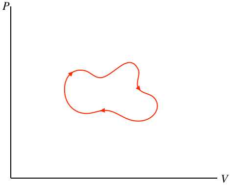
One of the state variables that returns to its original value when the cycle is complete is the internal energy. This means that for a full cycle we can use the first law to conclude:
0=ΔU=Q−W⇒Q=W
If there is a net amount of heat that comes into the system, it goes out of the system in the form of work – heat enters the gas, which in turn expands and does work on the piston. On the other hand, if a net amount of heat exits the system, it must have entered in the form of work. We can in fact even draw a general conclusion about which of these is occurring (and how much energy has been converted), based on the direction of the cycle (clockwise or counterclockwise) in the PV diagram. Whichever direction the cycle goes, part of the process is going left-to-right, and the rest is going right-to-left. The section of the process that is higher has a greater area under the curve, so if the top section is left-to-right there is net work done by the gas, and if it is right-to-left there is net work on the gas. Furthermore, the difference in the right-going and left-going processes is the net work done, and this is the area bounded by the cyclic loop.
Figure 6.1.2 – Work Done in a Cyclic Process is the Area Bounded by the Cycle
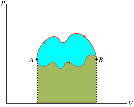
In the figure above, the area under the upper portion of the curve is positive, and the area under the lower portion is negative, so the total area for the full process is the difference, which is the blue region enclosed by the loop defining the cycle. Notice that for the case shown, the total area is positive, and if the cycle went the other way then the net work would be negative. We therefore conclude:
- the area inside a closed cycle loop in a PV diagram represents the net amount of energy converted between work and heat
- clockwise cyclic processes on the PV diagram represent physical systems for which heat is entering and an equal amount of work is done by the gas
- counterclockwise cyclic processes on the PV diagram represent physical systems for which work is done on the gas and an equal amount of heat is expelled by the gas
Example 6.1.1
The cyclic process of an ideal gas shown in the PT diagram below is rectangular, with vertical and horizontal sides at the positions labeled.

- Find the total heat transferred during the full cycle in terms of the quantities labeled, and indicate whether the heat is transferred into or out of the system.
- Sketch the PV diagram of this cyclic process.
- Solution
-
a. As this is not a PV diagram, the total work done or heat exchanged is not simply the area inside the closed shape. We therefore need to look at each segment individually. The horizontal segments are processes that maintain a constant pressure, so they are isobaric. We know the work done during such a process in terms of the temperature change from Equation 5.8.9: Q=nCPΔT. The two isobaric processes involve equal/opposite temperature changes, so these heat exchanges cancel each other out. The vertical segments are processes that maintain a constant temperature, so they are isothermal, and we can write down the work done for each segment using Equation 5.8.16:
leftsegment:Q=nRT1ln[P1P2]rightsegment:Q=nRT2ln[P2P1]}⇒Qtot=nRT2ln[P2P1]+nRT1ln[P1P2]=nR(T2−T1)ln[P2P1]
b. We need to sketch two isobaric and two isothermal processes that form a closed loop in a PV diagram. The isotherms need to be hyperbolas, which means the upper corners need to be at lower volumes than the corners directly below them on the PT diagram. Also, the work done in the upper isobaric process has to be equal in magnitude to the work done in the lower isobaric process (since we found that they cancel in part a). But the upper process is at a higher pressure, so the volume change has to be smaller (i.e. the horizontal segment is shorter on top than on bottom).
