
5.4: Modes of Heat Transfer


- Last updated
- Nov 8, 2022
- Save as PDF

( \newcommand{\kernel}{\mathrm{null}\,}\)
Conduction
We know the effects of heat being transferred into or out of systems, but now we are going to take a look at the ways in which this transfer can occur. As we stated earlier, “heat” is a rather generic description of energy transfer due to a temperature difference between two systems, and we will see there are three modes through which this transfer can occur. The first is the most intuitive, and as it turns out, the one we can most easily deal with mathematically. It is called conduction.
As we saw with thermal expansion, the trick to understanding conduction is to consider what is happening on a microscopic scale. Consider a solid cylindrical object that connects two systems at different temperatures. This cylinder acts as the conduit for heat energy to flow from the hotter system to the cooler one. We model this cylinder microscopically using parallel chains of particles joined by springs.
Figure 5.4.1 – Heat Conductor Model
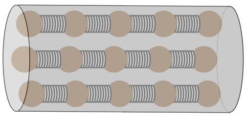
[Technically, these particles should be attached to all of their nearest neighbors by springs, but we will only be looking at the transfer of the heat along the length of the cylinder, so we have simplified the model accordingly.]
It should be clear from this model how heat energy can be transferred from one end of the cylinder to the other: If we vibrate the particles on one end of the cylinder, they will vibrate their nearest neighbors, and the effect will carry its way down to the other end. This is easy to see, but what is tougher to understand is that we will be considering only steady-state circumstances, which means that the particles on each end of the cylinder vibrate with amplitudes that have energies that match the systems with which they are in contact (these regions are called thermal reservoirs, because during the heat transfer process their temperatures don’t change appreciably). Every particle between the ends vibrates with an amplitude between the two extremes defined by the hot and cold reservoir.
Okay, so our task now (as it will be with all forms of heat transfer) is to determine the rate at which energy is transferred from one system to another in terms of the conditions provided. We'll do this by considering each element of this model in turn. As with any analysis of a continuously-changing phenomenon, we start with differential elements. In this case, we have two small segments of the cylinder at slightly different temperatures, across which some heat is transferred.
Figure 5.4.2 – Differential Heat Conduction

The more chains of spring-connected particles we can use, the faster the energy can be transferred. The number of chains is proportional to the cross-sectional area of the cylinder, so the rate of heat transfer is also proportional to the cross-sectional area:
dQdt∝A
The next factor in determining the rate of heat flow between these two segments is the temperature difference. It should not be surprising that heat will flow faster when the difference in temperature is greater. It turns out that the rate of heat flow is directly proportional to the temperature difference. This phenomenon is often referred to as Newton's law of cooling, and works fairly well as an approximation in more general circumstances, though it is only strictly applicable to this one. We have to be careful about the sign we use; recall that the sign for dQ is positive when heat is flowing into a system, but in this case the heat is flowing out of the system with the higher temperature:
dQdt∝−dT
In order to get all the energy in the first segment to be transferred into the second segment, energy in the left end of the segment has to traverse the length of that segment, dx. The longer this segment is, the longer it will take, so the rate of heat transfer is inversely-proportional to that distance:
dQdt∝1dx
Different substances will be structured differently (different springs, different masses of particles, etc.), so we have to take into account the type of substance. We do that by incorporating that into the constant of proportionality (thermal conductivity, k) that turns the proportional relationships into an equality:
dQdt=−kAdTdx
The derivative of the temperature is called the temperature gradient, and can be thought of as the steepness at which the temperature tapers-off from the origin of the heat transfer (the hotter thermal reservoir) to its destination (the cooler thermal reservoir), which in the most general cases (e.g. in non-steady-state situations) will not be constant. This is known as the heat equation, but really it is a specific example of the diffusion equation, which applies to many other phenomena as well.
It turns out that this equation is overkill for our purposes (we are not about to start solving differential equations), and in fact in all the cases we address we will deal with steady-state situations with the temperature gradient being linear. When the temperature changes linearly from the hot thermal reservoir to the cool one, the gradient is a constant, equal to simply the temperature difference of the two reservoirs (ΔT), divided by the distance separating them (L):
dQdt=−kALΔT
Example 5.4.1
An iron bar with a square cross-section is used to melt square holes in a slab of ice. The bar is then cut in half and the two halves are welded together on their sides to make a new shorter bar with a rectangular cross-section. If the mass of ice melted in 10 minutes by the original bar is M, how much ice will be melted in 10 minutes by the new configuration? Assume the temperature on the hot end of the bar is the same in both cases.
- Solution
-
The rate of heat conduction is proportional to the cross-sectional area and inversely proportional to the length of the material through which the heat passes, and in this case the area doubles while the length is divided in half. The material is the same (thermal conductivity is unchanged), so the rate of heat flow is quadrupled. With four times as much energy transferred into the ice in the same period of time, four times as much ice is melted, so the answer is 4M.
Convection
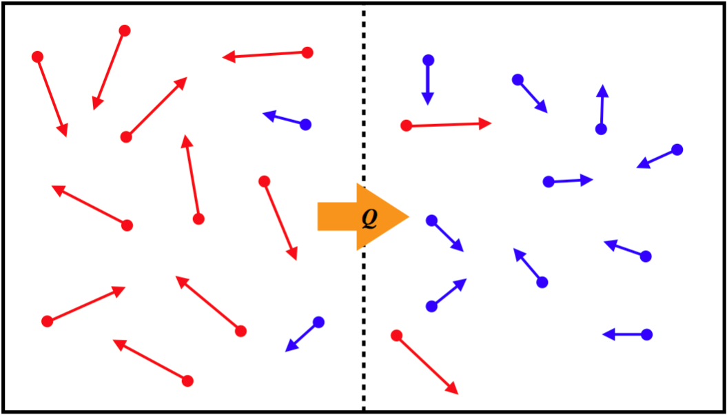
Convection is another form of heat transfer, that operates through a completely different mechanism from conduction. Rather than particles interacting with each other, the energy is transferred by simply having particles with more KE move (thanks to random motion) from the hotter region to the cooler one, while lower-KE particles take their place in the hotter region (there is no net exchange of particles), resulting in a transfer of energy.
Figure 5.4.3 – Convection Mechanism
Applying rigorous analysis to derive a mathematical model for the rate of heat flow via convection is well beyond the scope of this course. But an approximate relation based on the temperature difference of the two reservoirs is:
dQdt∝[ΔT]54
Two things to note here:
- While this doesn’t quite follow “Newton's Law of Cooling” like conduction, it comes very close.
- We don’t have the constant of proportionality, or even what this constant depends upon. That doesn’t mean this isn’t useful, because we can still compare the convection rates for two scenarios where “all else is equal.”
Without being more specific about the proportionality constants for conduction and convection, it is nevertheless a safe bet to say that convection in general is a faster mode of heat transport. For example, if you have a plastic bag full of hot water and a plastic bag full of cold water, and you want two plastic bags of warm water (so you want to transfer heat from the hot bag of water to the cold bag of water), the fastest way to achieve that is by mixing the water from the bags together, rather than by bringing the bags in contact with each other.
Radiation
The third way in which heat transfer can occur should become obvious when one thinks about how our Earth stays warm. After all, it is in contact with the vacuum of space (which in the absence of a nearby sun is at a temperature of 3K), so heat should be transferring out of it at an alarming rate. The source of the Earth’s incoming heat transfer is of course the Sun. But the space between the Sun and Earth is not conducting heat (it’s empty space - no particles connected with springs), and the Sun isn’t firing really hot particles to mix with the Earth’s atmosphere (well actually it is, but that “convection” is not doing much to heat our atmosphere, though it puts on a nice light show at the poles). Instead, the Sun is transferring energy to the Earth via radiation.
We already know that radiation is just light waves. We also know that light waves are driven by vibrating electric charges (electrons). One source of vibrating charges is atoms in a sample with thermal energy. The hotter the sample gets, the more energetically the charges vibrate, which means more energy is sent out in the form of radiation, so we would expect the electromagnetic power output of a sample to grow as its temperature grows, but it is by no means obvious in what way the power output will mathematically depend on the temperature.
These light waves don’t know where they are going, they only know that some vibrating electrons are driving them, so it is not the temperature difference that is causing this heat transfer, but rather the absolute temperature. A fellow named Boltzmann derived the dependence of the power output on temperature, and a guy named Stefan measured it. It turns out that the power output goes as the fourth power of the absolute temperature. The actual power output also depends upon the surface area (more space for the radiation to come out of), and a property called emissivity, which measures how well the surface emits light (how rough/smooth the surface is, how it is shaped, etc.) into the region just outside the object (the surface is the border between these two regions):
|dQdt|=σeAT4,σ≡5.67×10⁻⁸Wm2K4
The constant σ is called the Stefan-Boltzmann constant, e is the emissivity, and A is the surface area of the emitting body. The absolute value is included here because this equation involves the absolute temperature rather than a temperature difference. The sign we put to this equation depends upon whether we are talking about the rate at which heat that is exiting the object at temperature T (in which case the sign is negative), or the rate at which heat is entering the region surrounding the object at temperature T (in which case the sign is positive).
Nowhere here have we mentioned the frequency of the light emitted. It turns out that all of the frequencies (up to a certain maximum) are emitted, but the energy transferred is not uniform across frequencies. Remember, these thermal electrons are vibrating randomly, although that randomness has a non-uniform distribution, making some frequencies more common than others. Most of the light emitted in this manner at “everyday” temperatures (say, hundreds of kelvins) is in a part of the spectrum that we refer to as infrared, a frequency range we are unable to see with the naked eye, though we can see it with the help of special devices (e.g. infrared cameras). The part of the power output that is in the visible spectrum is too low for us to be able to see when the temperature is at “typical” temperatures in the region of 300K. But if something gets significantly hotter, the power output of every frequency goes up, and power in the visible spectrum can reach a level that we can see – the object “glows hot.”
Recall we said that heat transfer requires a temperature difference to occur, but here we seem to be saying that heat is transferred out of an object at an absolute temperature. Well, any object that can emit light can also absorb it. So let’s consider an object sitting in an environment which is at a different temperature.
Figure 5.4.4 – Heat Transfer to/from Surroundings Via Radiation

The emissivity is a property of the boundary surface between the two realms exchanging heat (which in this case we are calling the object and its surroundings), so naturally it is the same value going in both directions (we'll see another reason that this must be the case shortly). Obviously the surface area of the boundary is also the same going both ways as well. So the only thing that makes the heat energy exiting the object different (and entering the surroundings) from the heat energy going the other way (from surroundings to object) is the difference in temperature. We can now employ the sign convention for heat and conclude that the net rate of heat entering the surroundings is:
dQdt=σeA(T4−T4S)
Once again we see that net heat flow is induced by a difference in temperature, though like convection, this mode does not obey Newton's law of cooling.
Example 5.4.2
A typical red giant star is so big that it can fit about 1,000,000 stars the size of our sun inside of it (i.e. red giants occupy a volume about 1 million times greater than the volume occupied by our sun). For our sun to radiate energy at the same rate as such a star, how would their temperatures need to compare?
- Solution
-
One million times the volume translates into 100 times the radius, which in turn translates into 10,000 times the surface area. The rate of energy transfer due to radiation is proportional to the surface area, so if the temperatures were equal, the red giant would radiate energy at a rate 10,000 times that of our sun. The rate of energy transfer due to radiation also goes as the 4th power of the temperature, so if the sun was 10 times hotter than the red giant (it turns out it is not, though it is close to twice as hot), then that would exactly compensate for the much greater surface area of the red giant.
Digression: Temperatures Near Stars
As seen in the example, a common application of the Stefan-Boltzmann law comes from the study of stars. But such cases do not involve two regions sharing a common surface border at different temperatures. That is, the space immediately outside the surface of the sun is not the same near-absolute-zero temperature that it is far outside the solar system. Intuitively it makes sense that at steady-state the temperature would gradually decrease from what it is at the surface of the sun, down to the ~3K temperature we see in deep space, but is there some way to compute this temperature gradient? It's clear it can't be linear as it is for conduction, because drawing a straight line from the 5800K temperature of our sun down to 3K many billions of light years away would mean that the earth is residing in space that has a temperature that is essentially the same temperature as the sun. Figuring out this temperature gradient is essential to finding planets around other stars that could support life, because the planets will be in approximate thermal equilibrium with the space around them, and we assume life can only be sustained within a certain temperature range (the so-called "Goldilocks zone").
To solve this problem, let's consider a star with radius Ro and surface temperature To. Next, construct an imaginary spherical surface centered at the center of the star, with a radius R. We wish to compute the temperature T evaluated at this surface. Treating the star as a blackbody, the rate at which energy is radiated from it is:
dQdt(star)=σ(4πR2o)T4o
Now let's imagine that we treat our imaginary surface as a radiator of energy – we don't even know about the star inside of it. Naturally it behaves like a blackbody, because none of the radiation that strikes it from outside is reflected (it is imaginary!), and a perfect absorber is exactly the definition of a blackbody. We can therefore compute the rate at which it radiates energy outward:
dQdt(sphere)=σ(4πR2)T4
But of course, all of the power that comes from the star passes through this surface, so the power emitted by the surface is the same as the power emitted by the star. Setting them equal and solving for T gives:
T(R)=√RoRTo
So we see that the temperature drops as the inverse-square-root of the distance from the star.