1.6: Gauss's Law

The Density of Field Lines

We have said that the strength of an electric field in a given region is represented by the density of the electric field lines in that region. First, it is important to note that technically there is an infinite number of field lines. When we draw a diagram with a finite number of field lines, it is easy to tell where they are closer together and farther apart. But even when we extend to an infinite number the idea of line density holds. We now seek to quantify this measure somewhat.

Whenever we talk about the density of some quantity, it always comes as some kind of ratio:

\[ \text{density} \equiv \dfrac{\text{amount of something}}{\text{volume or area or length that it occupies}}\]

If we want to measure a density of infinitely-long field lines, we cannot do it using a ratio with a volume (we cannot contain them in a volume). Instead, we do it with an area, by counting the number of field lines that "pierce" a surface, and divide it by the area of that surface. So for example:

Figure 1.6.1 – Counting Surface Piercings By Field Lines

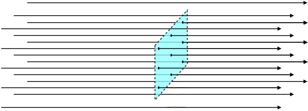
So in the case above, we would divide 9 piercings by the area of the rectangular surface to get the field line density. If we take the same rectangular surface elsewhere, and the field pierces it 18 times, we would conclude that the field is twice as strong there.

There is one problem with this scheme. We haven't specified the orientation of the surface relative to the field lines. For example, in the case above, if we rotate the rectangle slightly, we get a different number of piercings:

Figure 1.6.2 – Dependence of Surface Piercings on Surface Orientation

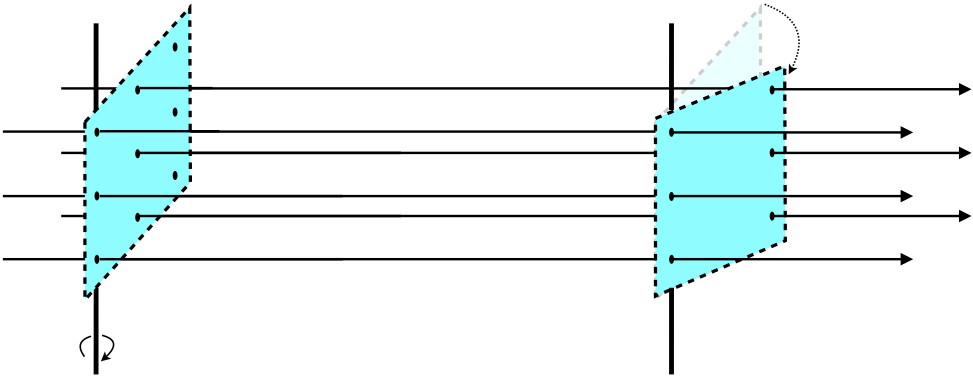
There is one unique way to define the density, and it results in the maximum number of piercings – define the density only in terms of a surface through which the piercings are perpendicular. So we define the field line density (which we equate to field strength) as follows:

\( \text{field line density} \equiv \dfrac{\text{number of field lines piercing a surface perpendicularly}}{\text{area of that surface}}\)

Notice that since there are infinitely-many field lines, we can define this surface to be as small as we like. We can then use an infinitesimally-small surface to probe various positions in space to determine the field strength at every point, provided we rotate it to be perpendicular to the field.

The Role of Charge

From the equation of the coulomb field, it's clear that the strength of the field is directly proportional to the amount of charge. That is, if we don't change the distribution of the charge, but just double the total amount everywhere (i.e. double the charge density everywhere it exists), then the field will look exactly like before, but it will be twice as strong. But we also measure field strength as density of field lines. If we use the same surface twice at the same point in space, once with the original charge, and once with double the charge, the density of field lines must double. Given that the field lines should not change direction, the only way that the field line density can double in this case is if the total number of field lines doubles. We therefore conclude that the number of field lines due to a collection of charge is proportional to the total amount of charge. For now we will write it this way:

\[Q = charge = \left(constant\right) \cdot \left(number\;of\;field\;lines\;coming\;out\;of\;it\right) = \mathcal C \cdot \mathcal N\]

There is a clever way that we can determine what this constant of proportionality is. It involves choosing a single positive point charge, and enclosing it at the center of of a spherical surface.

Figure 1.6.3 – Point Charge Enclosed by Two Spherical Surfaces

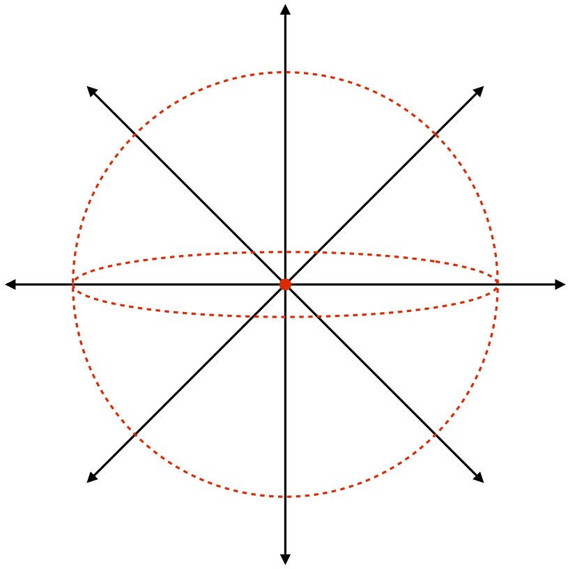
These field lines pierce the spherical surface perpendicularly, and the density of field lines is the same regardless of where you look on the surface of the sphere. Therefore the field line density is the number of field lines piercing the surface divided by the total surface area of the sphere (\(4\pi r^2\)). And since this surface completely encloses the charge, the number of field lines piercing the surface is the total number of field lines produced by that charge (\(\mathcal N\)). The field line density at this spherical surface is therfore:

\[density\;of\;field\;lines = \dfrac{\mathcal N}{4\pi r^2} \]

But the density of field lines is the electric field strength, which we happen to know at the surface of this sphere (a distance \(r\) from the point charge), from coulomb:

\[E\left(r\right) = \dfrac{Q}{4\pi \epsilon_o r^2} \]

Putting these last two equations tells us the number of field lines coming out of a charge \(Q\):

\[\mathcal N = \dfrac{Q}{\epsilon_o} \]

So we see that the constant of proportionality \(\mathcal C\) from Equation 1.6.2 is simply our old friend \(\epsilon_o\). Notice that it didn't matter what the radius of the sphere was. The number of field lines piercing the spherical surface is just however many are coming out of the charge \(Q\), and to get that number we just divide \(Q\) by \(\epsilon_o\). In fact, it didn't even depend upon the fact that we used a sphere at all. So long as we choose a closed surface that encloses the charge, the number of field line piercings will be the same – it depends only upon the amount of charge. With another surface, the field line density will differ from one place to the other on the surface, but the number of piercings won't change.

Electric Field Flux

We have been dancing around the issue of there being an infinite number of field lines. That is, the number of field lines coming from a charge \(Q\) is not really equal to \(\dfrac{Q}{\epsilon_o}\), any more than the electric field strength is really equal to the field line density. This is evident (if not conceptually) from the fact that the units don't match. So we need to drag our understandable-but-imprecise model into the world of more rigorous mathematics.

The link between these two worlds is the concept of electric field flux through a surface. In our description above, this is simply the number of field line piercings. But as we said, this is actually infinite, so we need the more mathematically rigorous definition of this term. We can get to this by relating the total number of piercings to the field line density.

Figure 1.6.4 – Definition of Electric Field Flux

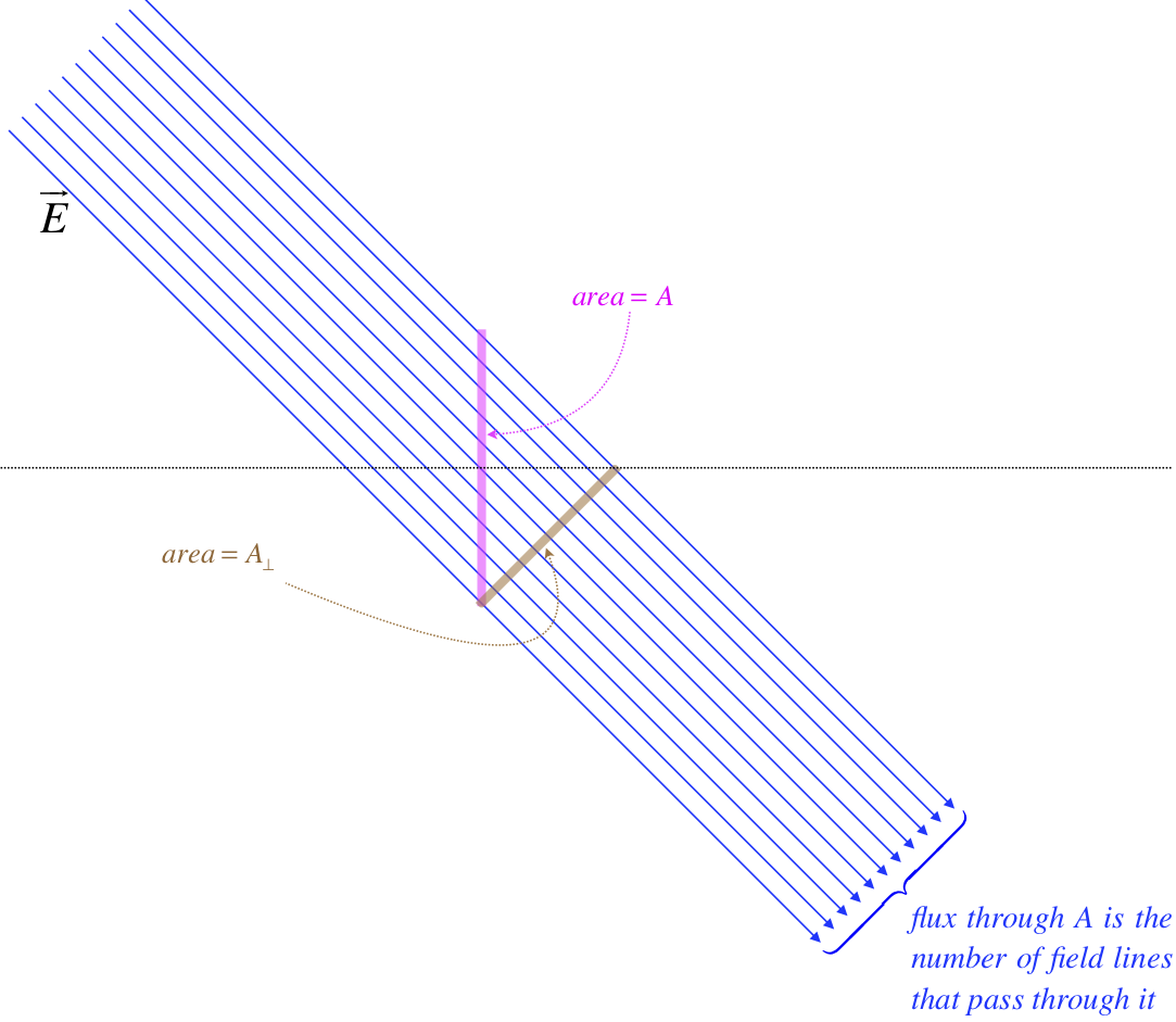
The number of field lines that pass through the pink surface with area \(A\) is equal to the number of field lines that pass through the brown surface with area \(A_\perp\). The number of field lines divided by \(A_\perp\) is the electric field strength, so if we call the electric field flux (i.e. the number of penetrating field lines) "\(\Phi_E\)," then we have:

\[E = \dfrac{\Phi_E}{A_\perp} \]

We can write this in terms of the original (pink) surface if we know the angle that the field makes with it. It is standard to measure this angle with a line perpendicular to that area (in the diagram above, that would be with the horizontal line shown). Doing the geometry reveals that the areas are related through the cosine of the angle, giving:

\[A_\perp = A\cos\theta \;\;\; \Rightarrow \;\;\; \Phi_E = E\;A\cos\theta \]

Now we are not always fortunate enough to have situations where we have a nice, flat surface and a uniform electric field with which to calculate the flux. When that is the case, we can only do small bits of flux at a time, and then add the small bits together to get the total flux.

Figure 1.6.5 – Differential Flux

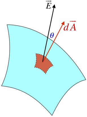
The differential area vector is defined with a magnitude equal to its area (which is infinitesimally small) and a direction that is perpendicular to the surface at that point on the surface. The electric field is also a vector, so when we compute the (tiny) flux through this area and we have to include the cosine of the angle, it's not surprising that we describe it with a dot product:

\[d\Phi_E = E\;dA\cos\theta = \overrightarrow E\cdot d\overrightarrow A \]

If we want to compute the flux over a finite surface, we have to add all of these infinitesimal contributions:

\[ \Phi_E\left(\text{surface}\right) = \int \limits_{\text{surface}} \overrightarrow E\cdot d\overrightarrow A \]

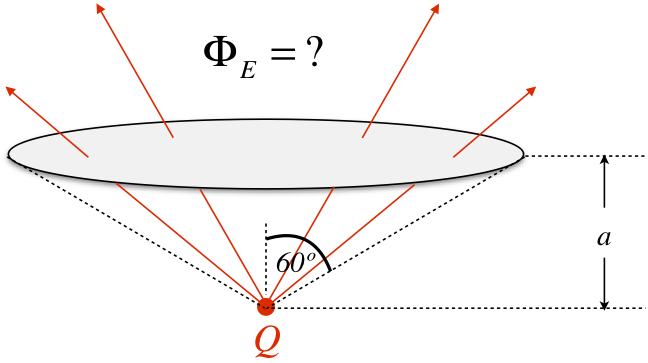
Example \(\PageIndex{1}\)

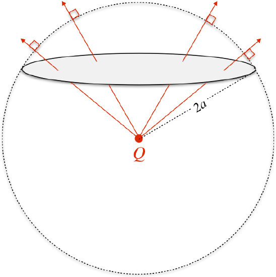
Find the flux of a point charge \(Q\) lying on the axis of a flat circular surface a distance \(a\) from the charge. The radius of the circular surface is such that a straight line joining the point charge and the edge of the surface makes a \(60^o\) angle with the axis (see the diagram below). Compute the electric flux through the surface.

Solution

We begin by computing the radius of the circular surface. The 30/60/90 triangle with the side opposite the \(30^o\) angle equal to \(a\) must have a hypotenuse equal to \(2a\), which gives it a longer side (the radius of the circular surface) equal to \(\sqrt 3 a\). We next need to come up with the flux through an arbitrary infinitesimal piece of the circle. Note that the electric field is not perpendicular to this surface everywhere, since it comes radially out of the point charge. At an arbitrary point on the circle, it looks like this:

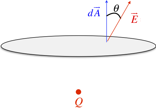
The simplest coordinate system to use here is cylindrical, with the \(z\)-axis being the line passing through the center of the circle and the charge. The distance out to the arbitrary position from the center is the cylindrical coordinate \(r\).

Trigonometry gives us the angle \(\theta\) in terms of \(a\) and \(r\):

\[\cos\theta = \dfrac{a}{\sqrt{r^2+a^2}} \nonumber\]

The magnitude of the electric field comes from coulomb:

\[ E=\dfrac{Q}{4\pi \epsilon_o \left(r^2+a^2\right)} \nonumber \]

A tiny section of area at the point in question in cylindrical coordinates is the usual (arclength multiplied by radial length):

\[dA = r\;dr\;d\phi \nonumber \]

Now put all of this together to compute the flux integral:

\[\Phi _E = \int \overrightarrow E \cdot d\overrightarrow A = \int E\;dA\cos\theta = \int \dfrac{Q}{4\pi \epsilon _o \left( r^2 + a^2 \right)} \left( r\;dr\;d\phi \right)\frac{a}{\sqrt {r^2 + a^2}} = \dfrac{Qa}{4\pi\epsilon_o} \int\limits_0^{2\pi} d\phi \int\limits_0^{\sqrt 3 a} \dfrac{r}{\left(r^2+a^2\right)^{\frac{3}{2}}} dr\nonumber \]

Integrating gives:

\[\Phi _E = \dfrac{Qa}{4\pi\epsilon_o}\left(2\pi\right)\left[\dfrac{-1}{\sqrt{r^2+a^2}}\right]_0^{\sqrt 3 a} = \boxed{\dfrac{Q}{4\epsilon_o}}\nonumber\]

Gauss's Law

The culmination of everything we have done in this section comes rather quickly by combining our revelations above with the mathematical definition of flux. We found that when we enclose a charge inside a closed surface, the number of piercings of that surface equals the total number of field lines produced by that charge, which we said was \(\dfrac{Q}{\epsilon_o}\). But the total number of piercings is also the flux through that surface. We therefore conclude that the total flux through a closed surface is given by:

\[ \oint\limits_{\rm{surface}}\overrightarrow E\cdot d\overrightarrow A = \dfrac{Q_{encl}}{\epsilon_o} \]

The integral with a circle in it is shorthand for "over a closed surface," and the subscript on \(Q\) indicates that the charge is enclosed in this surface. The direction of the vector \(d\overrightarrow A\) is out of the closed volume. This assures that the integral comes out positive for positive charges, and negative for negative charges. This is known as the integral form of Gauss's law. In the next section we'll look at the applications of this law.

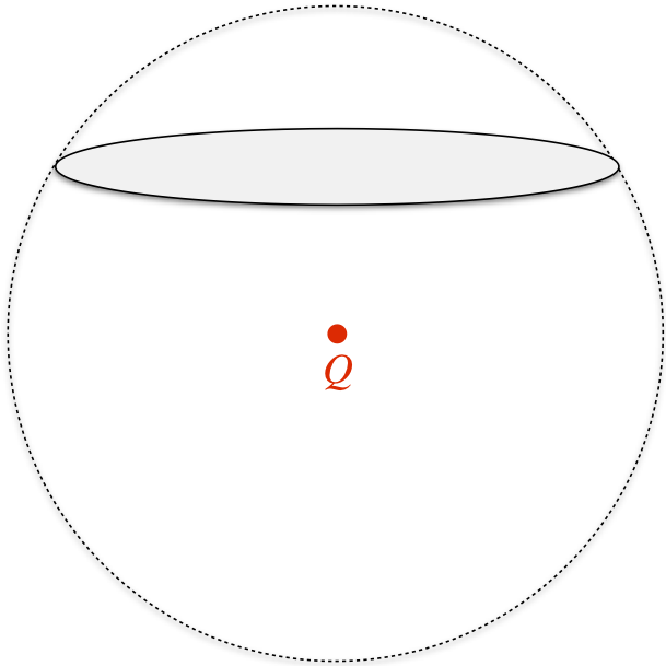
Example \(\PageIndex{2}\)

Repeat the flux calculation of the previous example, this time using Gauss's law with a closed sphere centered at the point charge and circumscribed around the surface, as shown in the diagram below.

Solution

We want to know the flux through the circular surface. The top section of the sphere (separated from the rest of the sphere by the circle) has no enclosed charge, so according to Gauss's law, the total flux out of its closed surface is zero. This means that the inward flux (coming through the circle from the charge) equals the outward flux (exiting the sphere in the top section). We can therefore determine the flux through the circle if we can compute the flux through the top section of the spherical surface.

The flux through the top section is easier to compute because the field lines are perpendicular to this surface and has the same magnitude everywhere. The infinitesimal area element in spherical coordinates is \(r^2\sin\theta\;d\theta\;d\phi\), where in this case \(r=2a\), so the flux integral is:

\[ \Phi_{circular\;surface} = \Phi_{top\;of\;sphere} = \int \overrightarrow E \cdot d\overrightarrow A = \int E\;dA\cos0^o = \int\int \dfrac{Q}{4\pi\epsilon_o\left(2a\right)^2}\;\left(2a\right)^2\sin\theta\;d\theta\;d\phi \nonumber\]

The limits of integration are pretty obvious: The azimuthal angle \(\phi\) goes all the way around ( \(0\rightarrow 2\pi\) ), while the polar angle \(\theta\) goes from vertical to the edge of the circle ( \(0\rightarrow 60^o\) ). The angular integrals are straightforward, and putting it all together gives the same answer as obtained previously.

If one happens to know that one quarter of the surface area of a sphere is subtended by a \(60^o\) solid angle (okay, so maybe not too many people have this information readily available), then the solution comes even faster. According to Gauss's law, the total flux out of the sphere is \(\frac{Q}{\epsilon_o}\), and since the charge is at the center of the sphere, the flux is uniform over the whole surface, which means that one fourth of the total flux must be going out of the top section, giving the answer immediately.

Example \(\PageIndex{3}\)

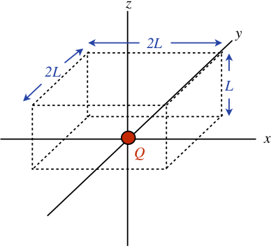
A point charge Q lies in the \(x\)-\(y\) plane. Consider an imaginary block (all vertices are right angles) with dimensions \(2L\times 2L \times L\), positioned with one of its square faces flat on the \(x\)-\(y\) plane, centered at the point charge (see diagram). Through a Herculean display of mathematical prowess, one can show via direct integration that the electric field flux through the top \(2L\times 2L\) surface comes out to be \(\dfrac{Q}{6\epsilon_o}\). Use Gauss's law to achieve the same result in a manner requiring far less effort.

Solution

 

Local (Differential) Form of Gauss's Law

Gauss's law can be cast into another form that can be very useful. There is a theorem from vector calculus that states that the flux integral over a closed surface like we see in Gauss's law can be rewritten as a volume integral over the volume enclosed by that closed surface. It is called the divergence theorem:

\[\oint\limits_{\rm{surface}} \overrightarrow E \cdot d\overrightarrow A = \int\limits_{\text{volume}\\ \text{enclosed}}\left(\overrightarrow\nabla\cdot \overrightarrow E\right) dV \]

Alert

It should be noted that this theorem is sometimes expressed a bit differently, particularly in mathematics texts. Namely, the differential area vector is broken into two parts – the magnitude \(dA\) and the direction \(\widehat n\) (a unit vector pointing perpendicularly out of the enclosed surface at the position where the area element is located), giving:

\[\oint\limits_{\rm{surface}}\overrightarrow E \cdot \widehat n \;dA = \int\limits_{\text{volume}\\ \text{enclosed}} \left(\overrightarrow\nabla\cdot \overrightarrow E\right) dV \nonumber \]

If we now apply this to Gauss's law, we get:

\[\dfrac{Q_{encl}}{\epsilon_o} = \int \left(\overrightarrow\nabla\cdot \overrightarrow E\right) dV \]

But we can write the charge enclosed in a volume in terms of the charge density \(\rho\) within that volume:

\[Q_{encl} = \int \rho\;dV \]

Comparing these last two equations suggests the following result:

\[ \overrightarrow\nabla\cdot \overrightarrow E=\dfrac{\rho}{\epsilon_o} \]

This is simply a restatement of Gauss's law, and is known as the local (or differential) form of that law.

This version can be used to solve the same kinds of problems as the integral form (though with a slightly different method), and is especially useful when the field's positional dependence is known (divergences are easier to compute than integrals).

Divergence Formulas

Now that it is clear that the divergence of the electric field is an important thing to be able to calculate, it is useful to point out some useful formulas for the divergence operation. The first of these is usable under all conditions:

Cartesian Coordinates

\[\overrightarrow\nabla\cdot\overrightarrow E\left(x,\;y,\;z\right) = \dfrac{\partial}{\partial x}E_x+\dfrac{\partial}{\partial y}E_y+\dfrac{\partial}{\partial z}E_z\]

The other two coordinate systems we will encounter frequently are cylindrical and spherical coordinates. In terms of these variables, the divergence operation is significantly more complicated, unless there is a radial symmetry. That is, if the vector field points depends only upon the distance from a fixed axis (in the case of cylindrical coordinates), or upon the distance from a fixed point (in the case of spherical coordinates), the divergence operation is fairly straightforward:

Cylindrical Coordinates

\[\overrightarrow\nabla\cdot\overrightarrow E\left(r,\cancel{\phi},\cancel{z}\right) = \dfrac{1}{r}\dfrac{\partial}{\partial r}\left(rE_r\right)\]

Spherical Coordinates

\[\overrightarrow\nabla\cdot\overrightarrow E\left(r,\cancel{\theta},\cancel{\phi}\right) = \dfrac{1}{r^2}\dfrac{\partial}{\partial r}\left(r^2E_r\right)\]

Example \(\PageIndex{4}\)

An electric field in a region of space near the origin can be expressed as:

\[E\left(x,y,z\right) = \alpha\;x\;\widehat i + \beta\left(y+y_o\right)^2\;\widehat j \nonumber\]

Show that if there is no charge at the origin, then the electric field there is equal to \(\dfrac{\alpha^2}{4\beta}\;\widehat j\) .

Solution

By Gauss's law, we have:

\[ \dfrac{\rho}{\epsilon_o} = \overrightarrow \nabla\cdot\overrightarrow E = \overrightarrow \nabla \cdot \left[ \alpha x\;\widehat i + \beta\left(y+y_o\right)^2\;\widehat j \right] = \dfrac{\partial}{\partial x}\left[\alpha x\right] + \dfrac{\partial}{\partial y}\left[\beta\left(y+y_o\right)^2\right] = \alpha + 2\beta\left(y+y_o\right)\nonumber \]

Zero charge at the origin means that the charge density vanishes there, so setting the density equal to zero at (\(x=y=z=0\)) gives:

\[0=\alpha + 2\beta y_o \;\;\; \Rightarrow \;\;\; y_o = -\dfrac{\alpha}{2\beta} \;\;\; \Rightarrow \;\;\; \overrightarrow E\left(x,y,z\right) = \alpha\;x\;\widehat i + \beta\left(y-\dfrac{\alpha}{2\beta}\right)^2\;\widehat j \nonumber\]

Plugging in (\(x=y=z=0\)) gives the desired answer.