6.1: From Light to Electrons

The Davisson-Germer Experiment

Light’s apparent dual nature as a wave and a particle might lead one to wonder, “If something we always thought was just a wave has particle properties, might not things we always thought to be particles have wave properties?” In our discussion of Compton scattering, we made an association between momentum and wavelength for light. Well, clearly particles like electrons have momentum, so maybe they have equivalent wavelengths, and therefore wave behavior. We'll explore this possibility with the results of series of experiments, accompanied by a particularly enlightening narrative first delivered by the late Richard Feynman.

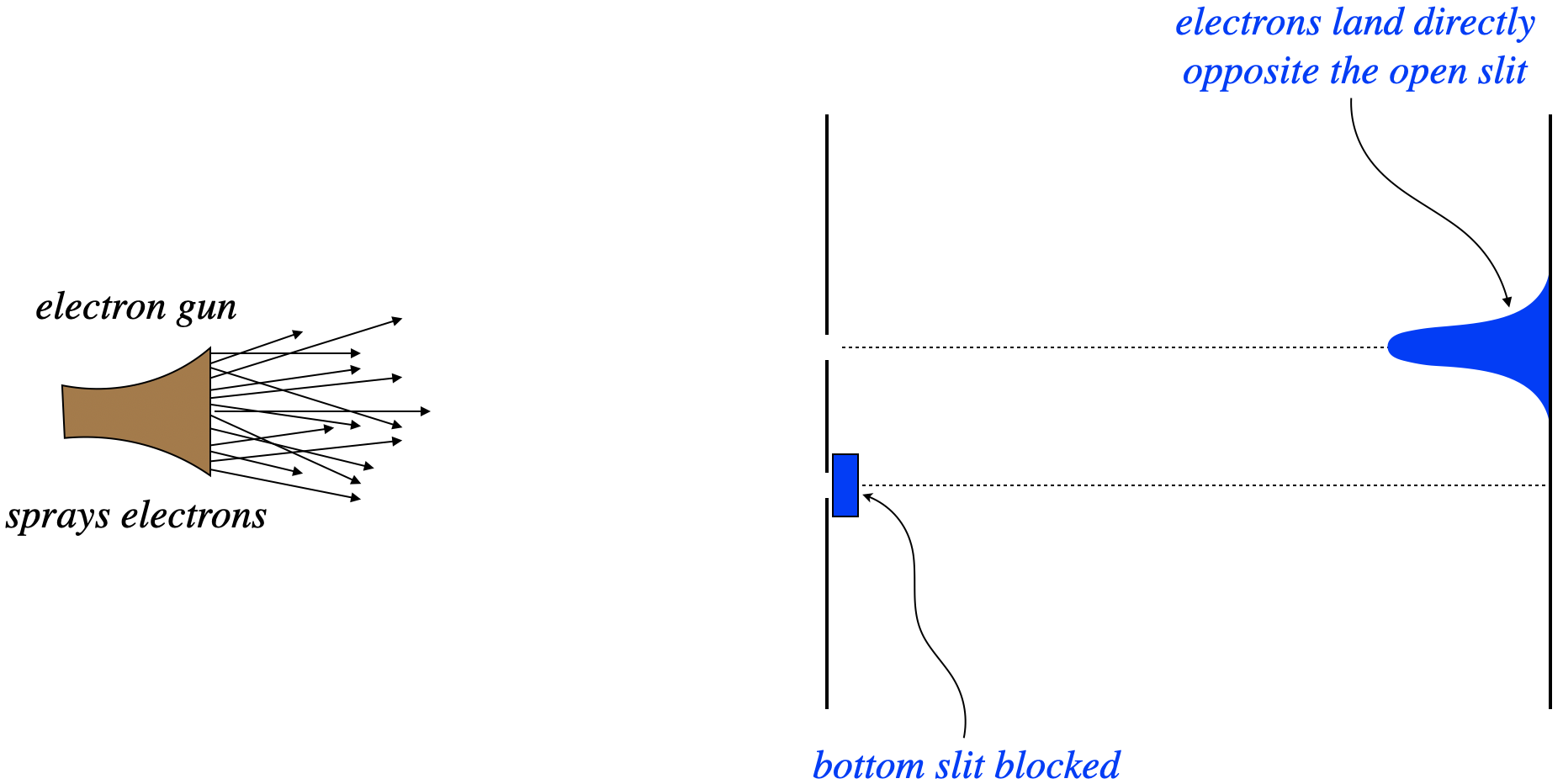
Consider firing electrons at a double-slit apparatus, with one of the two slits blocked. With one path to the screen, we see a distribution of electron-caused dots on the screen exactly as we would expect – in a cluster centered directly opposite the slit. Next the slits are reversed – the previously-closed slit is opened, and the previous open slit is closed. Unsurprisingly, we see the same result – a cluster of dots on the screen centered across from the slit.

Figure 6.1.1 – Electrons Through a Double Slit with One Slit Blocked

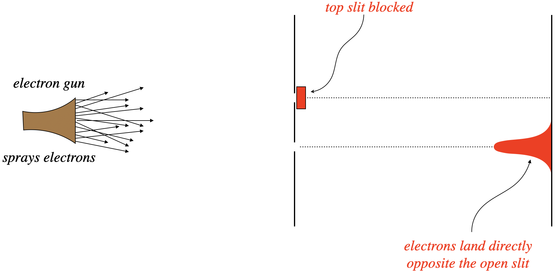
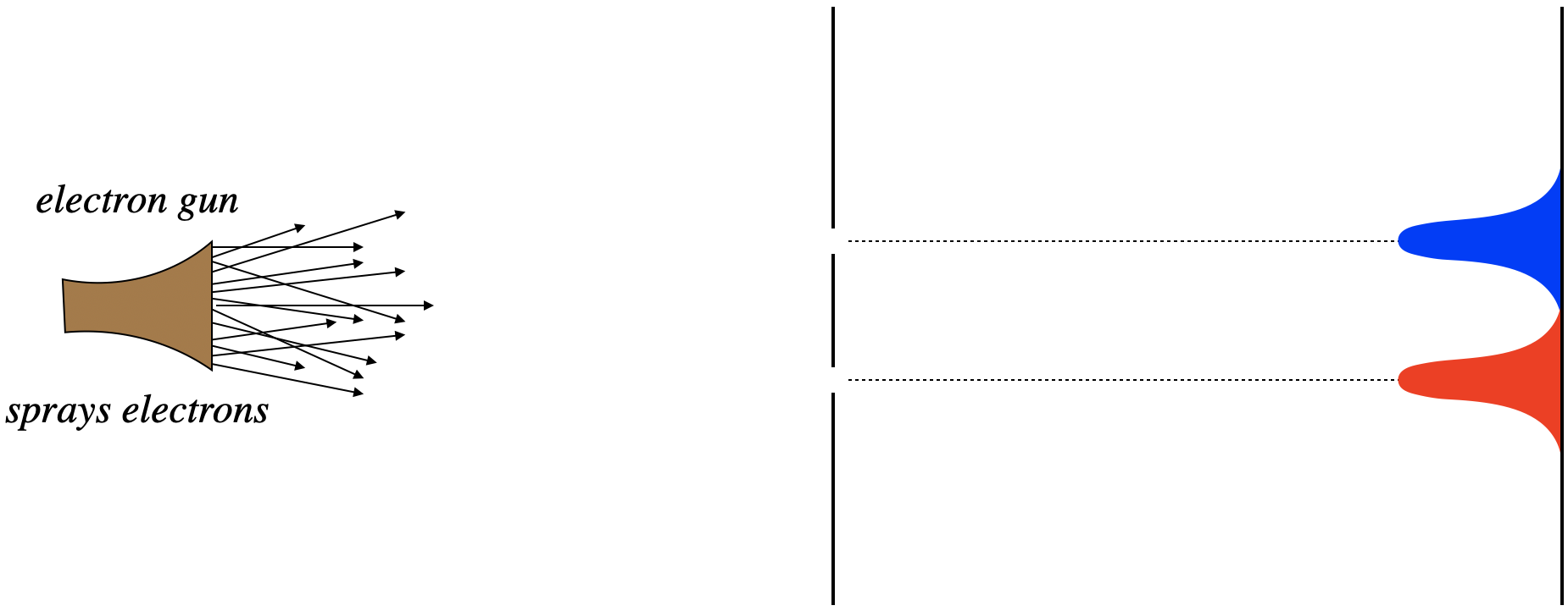
Given these results, the natural prediction of what happens when both slits are open is that we see both of the patterns we saw previously, at the same time. All the electrons that pass through the top slit should end up across from it, and all of those that pass through the bottom slit end up across that that slit.

Figure 6.1.2 – Electrons Through a Double Slit with Both Slits Open (Expected)

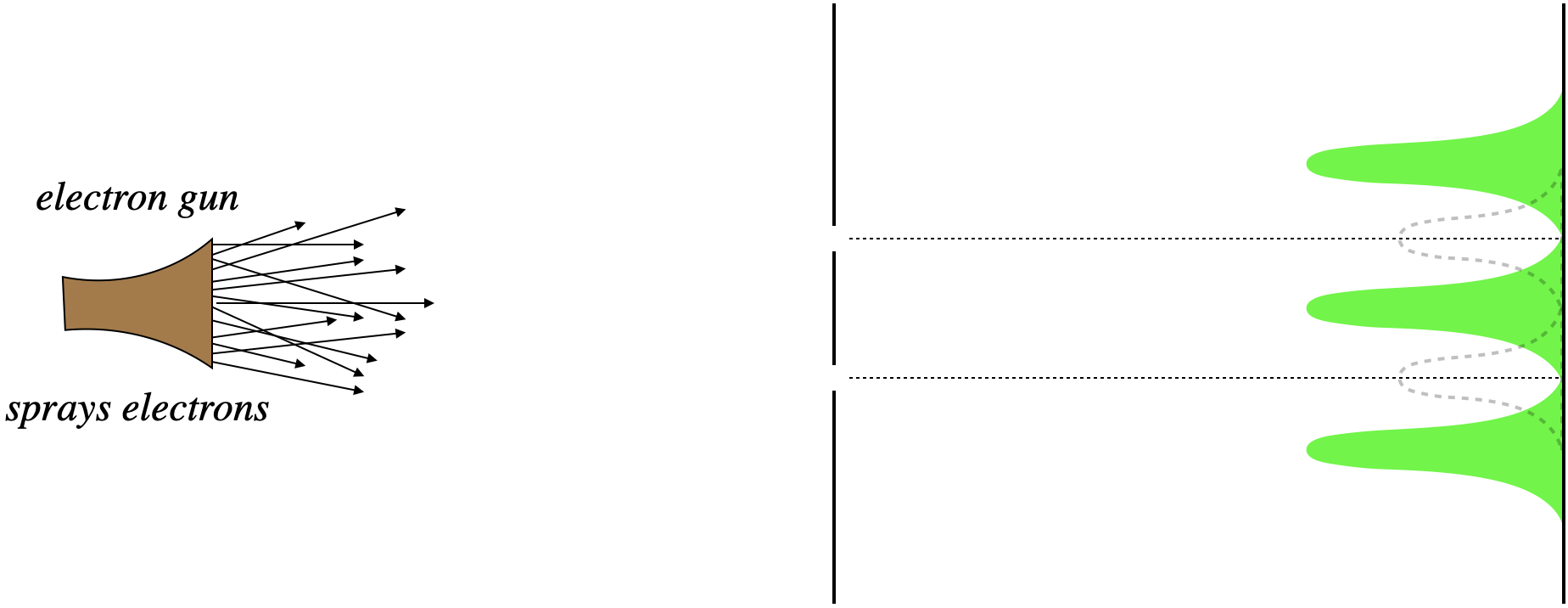
But the result (if the slits are spaced appropriately), is completely different. Rather than clusters of dots across from the slits, there are virtually no dots at all, and places where we expected very few dots are quite populous. In short, we see an interference pattern!

Figure 6.1.3 – Electrons Through a Double Slit with Both Slits Open (Actual)

The first attempt to explain this is naturally to say that the electrons are interacting with each other after they pass through the slits. But like the case of photons discussed in the previous section, the interference pattern emerges even if the electrons are sent through one at a time, once all the electron landings have occurred.

So the puzzling question is, "How does an electron, while going through the bottom slit, know whether or not the top slit is open?" If it is open, it's destination is different than if it is closed, but how can it tell where is is "supposed" to go? Like the case of photons, we can only conclude that the electron somehow passes through both slits at once, in the form of a wave. But that wave is not like any other wave, in that it carries information about the probabilities of landing at various points on the screen. This "probability wave" has the usual wave property that it can interfere with itself, creating some positions of zero probability, and others of relatively high probability, and these probabilities reflect the populations of the electron landing dots.

In an attempt to solve this puzzle, we might try to simply watch the electrons as they pass through the slits. To do this, let’s put a bright light source between the slits, so that when electrons pass, by the light scatters off them and we see a small flash of light coming from the location of the electron, thereby telling us which slit it went through.

Figure 6.1.4 – Watching the Electrons as They Pass Through the Slits

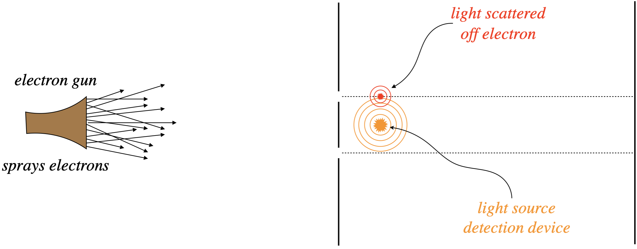
When we do this, we find we have a problem.  The interference pattern disappears, and the previous “expected” pattern of electrons landing either opposite one slit or the other emerges.  Apparently we have affected the motion of the electrons after they pass through the slit with our detection device.  But of course we have!  Light has momentum, and when we scatter it off the electrons, the momenta of the electrons are altered, apparently ruining the interference effect we were trying to study.  So the obvious solution?  Use light with less momentum, so that it doesn’t transfer so much to the electrons.  The means we have to use light of long wavelengths.

According to Compton scattering, the scattered light always has a longer wavelength than the light sent in, so we will be looking at very long wavelength light coming from the electron flashes.  The flashes are separated by a distance roughly equal to the slit separation, and we find that the effect of the light on the interference pattern starts to diminish when the wavelength of the light we use gets longer than the slit separation.  But then something new becomes a problem for our experiment. To determine where the light flash occurs, we need the light to carry with it some information about the distance scale – the wavelength of the light is a rough measure of the uncertainty of the position of its source. Just as we make the wavelength long enough for the interference pattern to return, it becomes too long to distinguish which slit the electron goes through. Infuriating... and amazing.

Comparing "Matter Waves" and Light Waves

We already have a mathematical description for light waves – Maxwell's equations. These don't explain why photons also act like particles, but one step at a time! Despite sharing the property of wave-particle duality, electrons and photons have some distinct differences, the two most notable being mass and electric charge. To keep these straight, we will employ the rather poor name of matter waves to describe the waves for electrons (and other particles), to distinguish them from light waves.

The fact that we get the same result for electrons as for light tells us that matter waves for free electrons (i.e. not under the influences of forces, like from electric or magnetic fields) must look very similar to those for light waves.  For light, we found (by utilizing our Physics 9B wave function skills in Physics 9C), the following expression for the time and position dependence of the electric field magnitude for a light wave moving in the \(+x\)-direction (we’ll choose phase equal to zero at \(x = 0\), \(t = 0\):

\[E\left(x,t\right)=E_o\cos\left[\frac{2\pi}{\lambda}x-\frac{2\pi}{T}\right]\]

Since we now know how this wave relates to physical properties of the photon (i.e. its momentum and energy), let’s rewrite it in terms of those quantities:

\[p=\frac{h}{\lambda},\;\;E=hf=\frac{h}{T}\;\;\;\Rightarrow\;\;\;E\left(x,t\right)=E_o\cos\left[\left(\frac{2\pi}{h}p\right)x-\left(\frac{2\pi}{h}E\right)t\right]\]

The quantity \(\frac{h}{2\pi} comes up frequently in quantum physics, so it is given its own symbol: \(\hbar\) (pronounced "h-bar"). This makes our expression for the electric field:

\[E\left(x,t\right)=E_o\cos\left[\frac{p}{\hbar}x-\frac{E}{\hbar}t\right]\]

We know that the matter waves and light wave functions should have the same form, because when it comes to interference, waves are waves.  So we expect that matter wave functions at least look similar to this.  But what about the wave equation?  We know that Maxwell showed that light waves can be described by the “usual” wave equation (again, simplifying to a wave traveling along the x-axis):

\[\dfrac{\partial^2E}{\partial x^2}=\frac{1}{c^2}\frac{\partial^2E}{\partial t^2}\]

It's easy to show that this wave equation works perfectly for light, because when we plug in our wave function from above, we get

\[\left.\begin{array}{l}\dfrac{\partial^2E}{\partial x^2}=-\left(\dfrac{p}{\hbar}\right)^2E\left(x,t\right) \\ \dfrac{\partial^2E}{\partial t^2}=-\left(\dfrac{E}{\hbar}\right)^2E\left(x,t\right)\end{array}\right\}\;\;\;\dfrac{\partial^2E}{\partial x^2}=\frac{1}{c^2}\dfrac{\partial^2E}{\partial t^2}\;\;\;\Rightarrow\;\;\;-\left(\dfrac{p}{\hbar}\right)^2=-\frac{1}{c^2}\left(\dfrac{E}{\hbar}\right)^2\;\;\;\Rightarrow\;\;\;E=pc\]

But as we saw in relativity, matter is very different from light – it has mass, and therefore this relationship between energy and momentum doesn’t hold for matter.  That means we need a different wave equation for matter waves than for light waves.

Schrödinger's Equation for Free Particles

We technically should find a wave equation for matter that satisfies the energy/momentum relation for relativity, but this turns out to be tougher to do mathematically, and historically this was not done, either.  Instead, we’ll assume that the particles we will be dealing with will be moving at speeds that are not relativistic, and we’ll use the Physics 9A-level relationship between kinetic energy and momentum:

\[KE=\dfrac{p^2}{2m}\]

Matter waves are not waves in electric and magnetic fields, so we need a symbol to describe the wave function, and the standard choice for this is the Greek letter psi: \(\psi\).  So for a freely-moving electron (we’ll deal with electrons under the influence of forces later), we need a wave equation that gives us the correct relation between energy and momentum, but still gives us a harmonic wave that interferes in the same way that a light wave does.  Notice that if our wave function has the same coefficients for \(x\) and \(t\) as for light, then we need two derivatives with respect to \(x\) (to give us the \(p\)-squared), but only one with respect to \(t\) (so that we get only one factor of \(E\)).  Also, each derivative brings out a factor of \(\hbar^{-1}\), so we need to multiply by a factor of \(\hbar\) for each derivative.  And finally, we need a factor of \(2m\) introduced into the denominator to construct the kinetic energy/momentum relation.  So let’s try this:

\[\dfrac{\hbar^2}{2m}\dfrac{\partial^2}{\partial x^2}\psi\left(x,t\right)=\hbar\dfrac{\partial}{\partial t}\psi\left(x,t\right) \\ \text{where:   }\psi\left(x,t\right)=\psi_o\cos\left[\dfrac{p}{\hbar}x-\dfrac{E}{\hbar}t\right]\]

The chain rules for the derivatives all work out nicely, but this wave equation falls short in the derivative itself – the derivative of cosine is (negative) sine, so while all the constants work out fine in front of the trig function, the trig functions themselves don’t match.

A guy named Erwin Schrödinger didn’t give up when he got this close.  He realized that just as light waves have two parts (electric and magnetic), so too should matter waves. Here’s how he incorporated two parts to the wave function: He allowed it to be a complex number.  The real part of the wave function would be one part of the matter wave, and the imaginary part another.  And just like for EM waves where changing electric fields give rise to magnetic fields and vice-versa, the real and imaginary parts of this wave function also mix.  His solution is now known as Schrödinger’s equation (for a free particle):

\[-\dfrac{\hbar^2}{2m}\dfrac{\partial^2}{\partial x^2}\psi\left(x,t\right)=i\hbar\dfrac{\partial}{\partial t}\psi\left(x,t\right) \\ \text{where:   }\psi\left(x,t\right)=\psi_o\cos\left[\dfrac{p}{\hbar}x-\dfrac{E}{\hbar}t\right]+i\sin\left[\dfrac{p}{\hbar}x-\dfrac{E}{\hbar}t\right]\]

We can shorten the formula for the wave function by using a famous identity attributed to Euler:

\[e^{i\theta}=\cos\theta+i\sin\theta\;\;\;\Rightarrow\;\;\;\psi\left(x,t\right)=\psi_oe^{i\left(\frac{p}{\hbar}x-\frac{E}{\hbar}t\right)}\]