1.2: Wave Properties

Periodic Waves

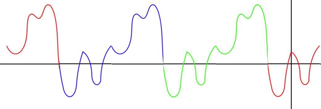
There are qualities that are not required of general waves which are nonetheless common features of waves encountered in nature. The most common special characteristic of a wave is when it continually repeats a specific waveform as it propagates. Such a wave is said to be periodic. There are a couple ways to determine if a wave is periodic. The first is to take a snapshot of the wave, and see if its waveform is repeated in space:

Figure 1.2.1a – Snapshot of a Periodic Wave

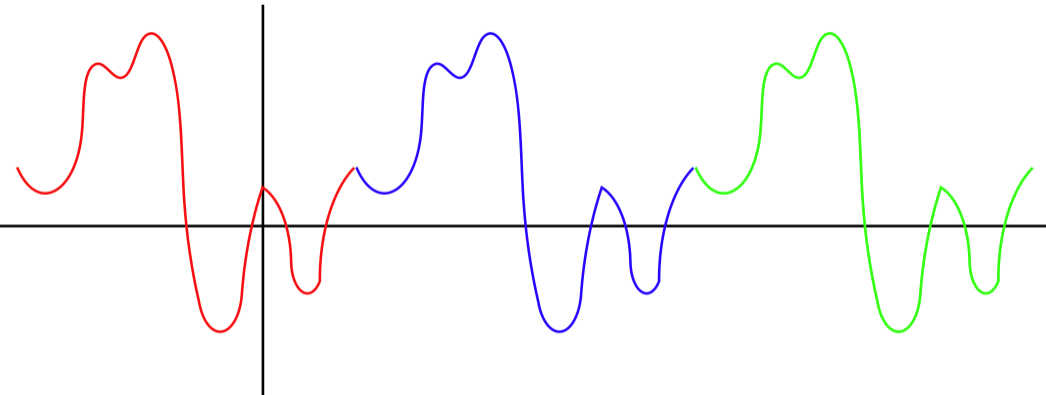
It should be noted that the starting point of each waveform in the diagram above was chosen arbitrarily. That is, if we look at the same snapshot of the wave as above, we could just as easily demonstrate its periodic nature with different segments:

Figure 1.2.1b – Snapshot of a Periodic Wave

The second way to determine if a wave is periodic is mathematical. The function repeats itself upon translation by a certain distance in the \(\pm x\) direction. That is:

\[f\left(x\pm vt\right) = f\left(x\pm vt \pm n \lambda\right),\;\;\;\;\;\;n=0,\;1,\;2,\dots\]

The quantity \(\lambda\) is the length of the repeating waveform, and is called the wavelength of the wave. A glance at the two diagrams above should make it clear that the wavelength is a universal feature of that particular wave, and does not depend upon where we choose the starting point to be.

The snapshot of the wave tells us something about its spatial features, but the wave is moving, so if we want to know something about its time-dependence, we need to select a specific point in space, and observe the displacement of the medium as the wave goes by. The wave moves at a constant speed, and the length of each repeating waveform is the same, so the time span required for a single waveform to go by is a constant for the entire wave, called the period of the wave. An alternative way of measuring the temporal feature of the wave is the rate at which medium displacements repeat, called frequency. Frequency is measured in units of cycles per second, a unit known as hertz (Hz). Since 1 period is the time required for one cycle, there is a simple relationship between these quantities:

\[f=\dfrac{1}{T}\]

We can make another association of periodic wave properties. If we pick a specific point on a waveform (called a point of fixed phase for the wave), and follow its motion, it should be clear that it travels a full wavelength in the time of one period. We therefore can relate the wave speed, wavelength, and period (or frequency):

\[v=\dfrac{\lambda}{T}=\lambda f\]

Wave Polarization

While the disturbance is not always a displacement of a medium, it always has a directional element to it. A wave that actually displaces a medium has an obvious direction: that of the displacement. Other waves have directional gradients that signify a direction. The direction in which the pressure is changing fastest (the pressure gradient direction) defines a direction for sound waves, and the direction of the electric field vectors defines a direction for light. This directional aspect of waves is also given a name: polarization. Generally the direction of medium displacement or gradient is compared to the direction of the wave's motion. There are two special cases that we will encounter for polarization of a wave:

transverse polarization: the medium's displacement or gradient is perpendicular to the wave’s direction of motion

Figure 1.2.2 – Transverse Wave

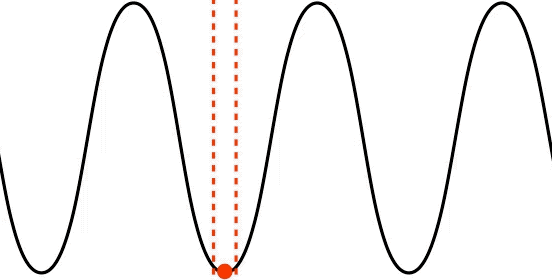
Note that the displacement of a single point in the medium (depicted by the red dot) is moving only vertically, while the wave moves horizontally. That these two motions are perpendicular to each other is the defining characteristic of a transversely polarized wave. Waves on strings and surface water waves are examples of this kind of wave. As noted earlier, not all waves involve the medium displacing (we will see some examples where this is the case later), but whatever fluctuation is occurring has a direction that can be compared with the direction of the wave's motion.

longitudinal polarization: the medium's displacement or gradient is parallel to the wave’s direction of motion.

Figure 1.2.3 – Longitudinal Wave

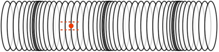
This time the displacement of a single point in the medium is parallel to the direction of the motion of the wave, the defining characteristic of a longitudinally polarized wave. Notice that like any other wave, the medium is not traveling with the wave, it is moving back-and forth. Physically these are waves induced by compressions (regions where the medium is more dense) and rarefactions (regions where the medium is less dense). These kinds of waves can be created in springs (as depicted above), but the most common physical example of this kind of wave is sound. Any medium (solid, liquid, or gas) will react to compression, and will therefore exhibit this kind of wave.

Alert

Snapshot graphs of waves of both kinds of polarization are sketched graphically with the displacement on the vertical axis and the position on the horizontal axis. When this is done, it "looks like" a transverse wave, but it is important to keep in mind that such a graph is not a picture of the wave. The vertical axis measures the displacement of the medium from the equilibrium point, which in the case of the red dot on the spring coil for the longitudinal wave in Figure 1.2.3 is the center of the horizontal dotted red lines.

Harmonic Waves

In the category of periodic waves, the easiest to work with mathematically are harmonic waves. The word "harmonic" is basically synonymous with "sinusoidal." For a one-dimensional wave, one might therefore assume that a harmonic wave function looks like:

\[f\left(x,t\right) = A\cos\left(x\pm vt\right)\]

While this comes close, it has a problem with units. The total phase of the wave function (the part in parentheses that is the argument of the cosine) cannot have any physical units, and this function has a phase with units of length. We can therefore repair this problem by dividing the phase by a constant of the wave that has units of length. The obvious such constant is the wavelength. So now our candidate wave function is:

\[f\left(x,t\right) = A\cos\left[\frac{1}{\lambda}\left(x\pm vt\right)\right]\]

This gets close, but if we are using radians as the measurement of phase, there is one more change we must add. If we consider a snapshot of this wave at \(t=0\), we would find that the sinusoidal waveform should repeat itself every time the value of \(x\) is displaced by \(\lambda\). If we are using radians as our angular measure, then this requires multiplying the phase by \(2\pi\). Then every change of \(x\) by \(\lambda\) will result in a change in the phase by \(2\pi\), and the function repeats itself properly. So we now have:

\[f\left(x,t\right) = A\cos\left[\frac{2\pi}{\lambda}\left(x\pm vt\right)\right]\]

There is one final addition to the phase that we need to make. Suppose we take a snapshot of the wave at \(t=0\) and look at the origin, \(x=0\). This function tells us that the value of the wave's displacement must be its maximum: \(A\). This is not a very general wave! To account for the possibility that the wave might have a different initial condition at the origin, we need to include a phase constant, \(\phi\). Distributing the factor of \(\frac{2\pi}{\lambda}\), and using Equation 1.2.3, we get the final form of the wave function of a 1-dimensional harmonic wave:

\[f\left(x,t\right) = A\cos\left(\frac{2\pi}{\lambda}x\pm \frac{2\pi}{T}t + \phi\right)\]

It is common to write this wave function in more compact ways. The first involves the definition of the wave number \(k\), and angular frequency \(\omega\):

\[k\equiv \frac{2\pi}{\lambda},\;\;\; \omega\equiv 2\pi f=\frac{2\pi}{T} \;\;\;\Rightarrow\;\;\;f\left(x,t\right) = A\cos\left(kx\pm \omega t + \phi\right)\]

Another definition that saves even more space is lumping the total phase of the wave into a single function variable: \(\Phi\left(x,t\right)\). It is clearly linear in the variables \(x\) and \(t\). That is:

\[f\left(x,t\right) = A\cos\left(\Phi\right),\;\;\;\;\;\; \Phi\left(x,t\right)=\frac{2\pi}{\lambda}x\pm \frac{2\pi}{T}t + \phi = kx\pm \omega t + \phi\]

Finally, it should be noted that although the cosine function was arbitrarily chosen here, we could have just as easily chose a sine function. The only difference between representing the wave with these two functions is the phase constant. That is, we can change from one function to the other if we change the phase constant by \(\frac{\pi}{2}\):

\[\cos\left(\Phi\right)=\sin\left(\Phi + \frac{\pi}{2}\right)\;\;\;\Rightarrow\;\;\; \phi\rightarrow\phi+\frac{\pi}{2}\]

Separation of Variables

The important thing to take away from the harmonic wave function in Equation 1.2.7 is that the wave has four constants of the motion that completely define it. Besides the wavelength, period, and phase constant, there is the amplitude, \(A\). All of these remain fixed in time, completely defining the wave that evolves thanks to its \(x\) and \(t\) dependence.  These constants can be extracted from what was referred to in the previous section as boundary conditions.

It turns out that harmonic wave functions have another feature that makes them special.  To see this, let's employ a powerful method that is used to solve equations like the wave equation called separation of variables.  We will not go into great detail here (you will see this used later in this course, and will see it over and over in future math and physics courses), but you will get a feel for how it works.  We will stick to the one-dimensional wave equation to keep it as simple as possible.

It goes like this: Let's look for solutions to the wave equation that satisfy a very specific criterion – let's assume the wave function can be separated into a product of two functions, one of them a function only of position, and the other a function of only time:

\[f\left(x,t\right)=\mathcal X\left(x\right)\cdot\mathcal T\left(t\right)\]

It should be immediately clear that only a special group of wave functions will satisfy this condition.  For example, \(f\left(x-vt\right)=\left(x-vt\right)^2\) is a one-dimensional wave function that cannot be written as a product of two functions with one of them only a function of \(x\) and the other only a function of \(t\).  Let's plug our special wave function into the wave equation:

\[\frac{\partial^2}{\partial x^2}f\left(x,t\right)=\frac{1}{v^2}\frac{\partial^2}{\partial t^2}f\left(x,t\right)~~~\Rightarrow~~~\frac{\partial^2}{\partial x^2}\left[\mathcal X\left(x\right)\cdot\mathcal T\left(t\right)\right]=\frac{1}{v^2}\frac{\partial^2}{\partial t^2}\left[\mathcal X\left(x\right)\cdot\mathcal T\left(t\right)\right]\]

Because of the nature of partial derivatives, the left side of this equation only takes two derivatives of the function \(\mathcal X\left(x\right)\), and the right side only two derivatives of the function \(\mathcal T\left(t\right)\).  These derivatives are of single-variable functions, so we don't even need to refer to them as partial derivatives when they act on the partial functions.  Representing ordinary derivatives with primes, we have:

\[\mathcal X''\left(x\right)\cdot\mathcal T\left(t\right)=\frac{1}{v^2}\mathcal X\left(x\right)\cdot\mathcal T''\left(t\right)\]

Dividing both sides of this equation by \(\mathcal X\left(x\right)\cdot\mathcal T\left(t\right)\) gives:

\[\frac{\mathcal X''\left(x\right)}{\mathcal X\left(x\right)}=\frac{1}{v^2}\frac{\mathcal T''\left(t\right)}{\mathcal T\left(t\right)}\]

And now for the magic... Notice that the left side of this equation is only a function of \(x\), while the right side is only a function of \(t\) (remember, \(v\) is a constant for the wave, and doesn't depend on either \(x\) or \(t\)).  The variables \(x\) and \(t\) are completely independent of each other – we can look at different positions on the wave at the same time, or at a single position on the wave at different times.  For two functions of independent variables to be equal to each other, it means that they must both equal the same constant.  For example, if the ratio on the left side of the equation depended on \(x\), then the right side would have to be a function of \(x\), and it is not.  Expressing this fact mathematically (and choosing a form of the constant that will make sense later), we have:

\[\frac{\mathcal X''\left(x\right)}{\mathcal X\left(x\right)}=\frac{1}{v^2}\frac{\mathcal T''\left(t\right)}{\mathcal T\left(t\right)}=-k^2\]

We can now write two separate equations, one exclusively in terms of \(x\), and the other exclusively in terms of \(t\) (thus the name of this method!):

\[\mathcal X''+k^2\mathcal X=0~~~~~~~~~~\mathcal T''+k^2v^2\mathcal T=0\]

These two differential equations are the same – they both involve two derivatives of a function equaling a constant times the function again.  What is more, we have seen this differential equation before! We know that either a sine or a cosine function will satisfy these equations, so a linear combination will as well.  We can therefore write solutions to these two equations as:

\[\mathcal X\left(x\right)=a\cos kx+b\sin kx~~~~~~~~~~\mathcal T\left(t\right)=c\cos \omega t+d\sin \omega t\]

[Here we have defined \(\omega\equiv kv\).]  So now we can reconstruct the full wave function:

\[f\left(x,t\right)=\mathcal X\left(x\right)\cdot\mathcal T\left(t\right)=\left(a\cos kx+b\sin kx\right)\left(c\cos \omega t+d\sin \omega t\right)\]

What this result says is that any wave of the given one-dimensional wave equation that can be separated into a product of two single-variable functions can be written in this form, and the specifics of that wave are given by the constants \(a\), \(b\), \(c\), \(d\), \(k\), and \(\omega\).  But there is one important restriction to keep in mind: The ratio \(\frac{\omega}{k}\) must equal the speed of the wave in question.

It is interesting to note that the basic cosine wave function given above in Equation 1.2.8 is not a separable solution to the wave equation. That is, one cannot reach Equation 1.2.8 (for given values of \(k\) and \(\omega\)) by an appropriate choice of the constants \(a\), \(b\), \(c\), and \(d\).  It can only be reached using a linear combination of two different separable solutions. We will cover this case in detail in a later chapter.