1.4: Curve Fitting

Many experiments require you to perform curve fitting. You have data points \[\begin{array}{c}X_1 \\ X_2 \\ \vdots \\ X_N \end{array} \begin{array}{c}Y_1 \\ Y_2 \\ \vdots \\ Y_N \end{array}\] which may be either direct measurement results, or derived from measurements. You are then required to fit these data to a relation such as \[Y = b_0 + b_1 X.\] The goal is to determine \(b_0\) and \(b_1\), which are called estimators.

Curve fitting, and the propagation of error into estimators, is a complicated subject within the mathematical discipline of statistics. For most experiments in this course, you will only need the most basic method, which is called weighted linear least squares regression.

In this method, each data point \((X_i,Y_i)\) is assigned a relative weight \(w_i\). Data points with smaller errors are considered more important (i.e., they have more “weight”). A standard weight assignment is \[w_i = \frac{1}{\Delta Y_i^{2}}. \label{weighting}\] Note that this ignores the errors in \(X\). There is no standard weighting procedure that accounts for errors in both \(X\) and \(Y\). So you should let the variable with more “relevant” error be the \(Y\) variable, so its error is used for the curve-fitting weights.

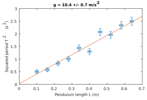
As an example, suppose we measure the period of a pendulum, \(T\), with varying arm length \(L\). Theoretically, \(T\) and \(L\) are related to the gravitational constant \(g\) by \[T = 2\pi \sqrt{\frac{L}{g}} \;\;\; \Rightarrow \;\;\; T^2 = \frac{4\pi^2}{g} \, L.\] We can fit our data to the relation \[T^2 = b_0 + b_1 L,\] and use \(b_1\) to estimate \(4\pi^2/g\). Hence, we can find \(g = 4\pi^2/b_1\), and its error \(\Delta g\): \[\frac{\Delta g}{g} = \frac{\Delta b_1}{b_1} \;\;\;\Rightarrow\;\;\; \Delta g = \frac{4\pi^2\Delta b_1}{b_1^2}.\] Suppose all our measurements of \(T\) have the same measurement error \(\pm \Delta T\). From the error propagation rule for powers (Section 3), \[\frac{\Delta (T^2)}{T^2} = 2 \frac{\Delta T}{T} \;\;\;\Rightarrow \;\;\; \Delta (T^2) = 2\,T\,\Delta T.\] Thus, the errors in \(T^2\) are not uniform: data points with large \(T\) have more error.

Sample Python program

A sample Python program for weighted linear least squares curve fitting is shown below. The fitting is done by the curve_fit function, from the scipy.optimize module.

In this program, curve_fit is called with four inputs: the model function, the \(x\) data, the \(y\) data, and the standard errors of the \(y\) data. The first input is a function that you must define, telling curve_fit what kind of curve to fit to (in this case, a first-order polynomial). The last three inputs are arrays of numbers.

The curve_fit function returns two outputs. The first output is an array of estimators (i.e., the additional inputs that, when passed to the model function, give the best fit to the data). The second output is a “covariance matrix”, whose diagonal terms are the estimator variances (i.e., taking their square roots yields the standard errors of the estimators).

from scipy import *
from scipy.optimize import curve_fit

## Input data (generated by simulation with random noise).
L = array([0.10, 0.16, 0.22, 0.28, 0.34, 0.40, 0.46, 0.52, 0.58, 0.64])
dL = array([0.01, 0.01, 0.01, 0.01, 0.01, 0.01, 0.01, 0.01, 0.01, 0.01])
T = array([0.71, 0.76, 0.91, 1.00, 1.20, 1.14, 1.44, 1.40, 1.53, 1.58])
dT = array([0.05, 0.05, 0.05, 0.05, 0.05, 0.05, 0.05, 0.05, 0.05, 0.05])

Tsq = T**2             # Estimates for T^2
Tsq_error = 2*T*dT     # Errors for T^2, from error propagation rules

## Define an order-1 polynomial function, and use it to fit the data.
def f(x, b0, b1): return b0 + b1*x
est, covar = curve_fit(f, L, Tsq, sigma=Tsq_error)

## Estimators and their errors:
b0, b1 = est               # Estimates of intercept and slope
db0 = sqrt(covar[0,0])     # Standard error of intercept
db1 = sqrt(covar[1,1])     # Standard error of slope

g = 4*pi*pi/b1             # Estimate for g (computed from b1)
dg = (g/b1)*db1            # Estimate for standard error of g

## Plot the data points, with error bars
import matplotlib.pyplot as plt
plt.errorbar(L, Tsq, xerr=dL, yerr=Tsq_error, fmt=’o’)
plt.xlabel(’Pendulum length L (m)’, fontsize=12)
plt.ylabel(’Squared period T^2 (s^2)’, fontsize=12)
## Include the fitted curve in the plot
L2 = linspace(0, 0.7, 100)
plt.plot(L2, b0 + b1*L2)
## State fitted value of g in the figure title
plt.title("g = {:.1f} +/- {:.1f} m/s^2".format(g, dg), fontsize=12)
plt.show()

The resulting plot looks like this:

Figure \(\PageIndex{1}\)

Sample Matlab program

Here is a sample Matlab program for weighted linear least squares curve fitting. It uses the glmfit function from Matlab’s Statistics Toolbox.

L  = [0.10, 0.16, 0.22, 0.28, 0.34, 0.40, 0.46, 0.52, 0.58, 0.64];
dL = [0.01, 0.01, 0.01, 0.01, 0.01, 0.01, 0.01, 0.01, 0.01, 0.01];
T  = [0.71, 0.76, 0.91, 1.00, 1.20, 1.14, 1.44, 1.40, 1.53, 1.58];
dT = [0.05, 0.05, 0.05, 0.05, 0.05, 0.05, 0.05, 0.05, 0.05, 0.05];

Tsq = T.^2;              % Estimates for T^2
Tsq_error = 2*T.*dT;     % Errors for T^2, from error propagation rules

%% Fit L and Tsq with weighted linear least squares
wt = 1 ./ (Tsq_error.^2);     % Vector of weights
[est, dev, stats] = glmfit(L, Tsq, ’normal’, ’weights’, wt);

%% Estimators and their errors:
b0 = est(1);               % Estimate of intercept
b1 = est(2);               % Estimate of slope
db0 = stats.se(1);         % Standard error of intercept
db1 = stats.se(2);         % Standard error of slope

g = 4*pi*pi/b1;            % Estimate for g (computed from b1)
dg = (g/b1)*db1;           % Estimate for standard error of g

%% Plot the data points and fitted curve
errorbar(L, Tsq, Tsq_error, Tsq_error, dL, dL, "o");
xlabel("Pendulum length L (m)");
ylabel("Squared period T^2 (s^2)");
%% State the fitted value of g in the figure
title(sprintf("g = %.1f +/- %.1f m/s^2", g, dg));
%% Plot the fitted curve
L2 = linspace(0, 0.7, 100);
hold on; plot(L2, b0 + b1*L2); hold off;

The resulting plot looks like this:

Figure \(\PageIndex{2}\)

Curve fitting with Origin

The procedure for curve fitting with Origin is summarized below. For more details, consult the Origin online documentation.

1. Populate a worksheet with columns for (i) \(X\), (ii) \(Y\), and (iii) \(\Delta Y\). You can enter the numbers manually, or import them from an external file.

2. Select the menu item Plot→Symbol→ Scatter. Click on the appropriate boxes to specify (i) which column to use for the horizontal (\(X\)) variable, (ii) which column to use for the vertical (\(Y\)) variable, and (iii) which column to use for the error \(\Delta Y\).

3. Select the menu item Analysis→ Fitting→Linear Fit. In the dialog box, check that the right fitting options are entered. Under Under Fit Control→ Errors as Weight, ensure that the Instrumental option is chosen. This corresponds to the standard weighting scheme from Section 1.4. Once ready, perform the fit.

4. The fitted curve will be inserted automatically into the graph. By default, a Fit Results table is also automatically added; you can click-and-drag to move or resize this table, and double-click to edit its contents.

   By default, Origin makes the table too small to be legible, so you ought to increase the size. Also, you should omit any statistical quantities listed in this table that are not relevant to your data analysis (e.g., the Pearson’s \(r\)). Finally, you still need to convert the estimators into whatever quantities you are ultimately interested in (such as \(g\)).

The resulting plot looks like this:

Figure \(\PageIndex{3}\)

[1] I. G. Hughes and T. P. A. Hase, Measurements and their uncertainties (Oxford University Press, 2010).