Search

Text Color

Margin Size

Font Type

Enable Dyslexic Font

2.12: Principal Planes

Last updated

Mar 5, 2022
Save as PDF
- 2.11: Thick Lenses
- 2.13: The Lazy Way

$\newcommand{\vecs}[1]{\overset { \scriptstyle \rightharpoonup} {\mathbf{#1}} }$

$\newcommand{\vecd}[1]{\overset{-\!-\!\rightharpoonup}{\vphantom{a}\smash {#1}}}$

$\newcommand{\id}{\mathrm{id}}$ $\newcommand{\Span}{\mathrm{span}}$

( \newcommand{\kernel}{\mathrm{null}\,}\) $\newcommand{\range}{\mathrm{range}\,}$

$\newcommand{\RealPart}{\mathrm{Re}}$ $\newcommand{\ImaginaryPart}{\mathrm{Im}}$

$\newcommand{\Argument}{\mathrm{Arg}}$ $\newcommand{\norm}[1]{\| #1 \|}$

$\newcommand{\inner}[2]{\langle #1, #2 \rangle}$

$\newcommand{\Span}{\mathrm{span}}$

$\newcommand{\id}{\mathrm{id}}$

$\newcommand{\Span}{\mathrm{span}}$

$\newcommand{\kernel}{\mathrm{null}\,}$

$\newcommand{\range}{\mathrm{range}\,}$

$\newcommand{\RealPart}{\mathrm{Re}}$

$\newcommand{\ImaginaryPart}{\mathrm{Im}}$

$\newcommand{\Argument}{\mathrm{Arg}}$

$\newcommand{\norm}[1]{\| #1 \|}$

$\newcommand{\inner}[2]{\langle #1, #2 \rangle}$

$\newcommand{\Span}{\mathrm{span}}$ $\newcommand{\AA}{\unicode[.8,0]{x212B}}$

$\newcommand{\vectorA}[1]{\vec{#1}} % arrow$

$\newcommand{\vectorAt}[1]{\vec{\text{#1}}} % arrow$

$\newcommand{\vectorB}[1]{\overset { \scriptstyle \rightharpoonup} {\mathbf{#1}} }$

$\newcommand{\vectorC}[1]{\textbf{#1}}$

$\newcommand{\vectorD}[1]{\overrightarrow{#1}}$

$\newcommand{\vectorDt}[1]{\overrightarrow{\text{#1}}}$

$\newcommand{\vectE}[1]{\overset{-\!-\!\rightharpoonup}{\vphantom{a}\smash{\mathbf {#1}}}}$

$\newcommand{\vecs}[1]{\overset { \scriptstyle \rightharpoonup} {\mathbf{#1}} }$

$\newcommand{\vecd}[1]{\overset{-\!-\!\rightharpoonup}{\vphantom{a}\smash {#1}}}$

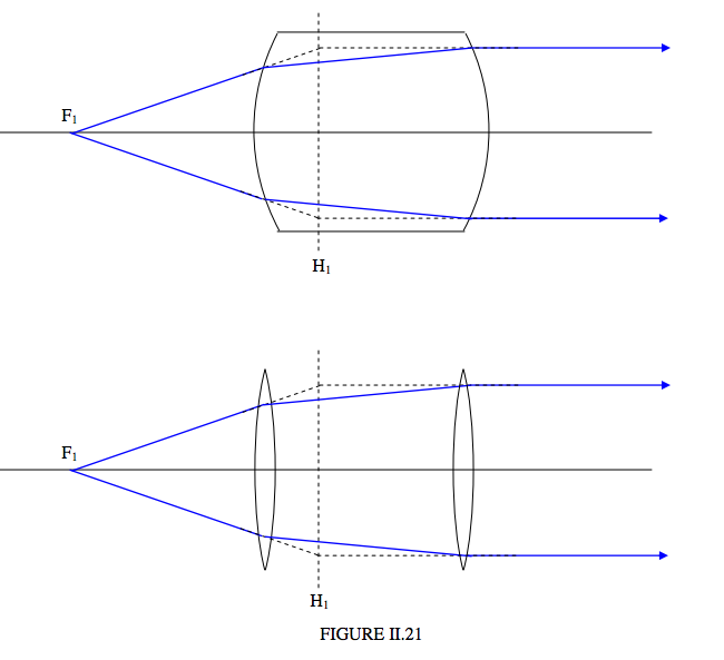
$\newcommand{\avec}{\mathbf a}$

$\newcommand{\bvec}{\mathbf b}$

$\newcommand{\cvec}{\mathbf c}$

$\newcommand{\dvec}{\mathbf d}$

$\newcommand{\dtil}{\widetilde{\mathbf d}}$

$\newcommand{\evec}{\mathbf e}$

$\newcommand{\fvec}{\mathbf f}$

$\newcommand{\nvec}{\mathbf n}$

$\newcommand{\pvec}{\mathbf p}$

$\newcommand{\qvec}{\mathbf q}$

$\newcommand{\svec}{\mathbf s}$

$\newcommand{\tvec}{\mathbf t}$

$\newcommand{\uvec}{\mathbf u}$

$\newcommand{\vvec}{\mathbf v}$

$\newcommand{\wvec}{\mathbf w}$

$\newcommand{\xvec}{\mathbf x}$

$\newcommand{\yvec}{\mathbf y}$

$\newcommand{\zvec}{\mathbf z}$

$\newcommand{\rvec}{\mathbf r}$

$\newcommand{\mvec}{\mathbf m}$

$\newcommand{\zerovec}{\mathbf 0}$

$\newcommand{\onevec}{\mathbf 1}$

$\newcommand{\real}{\mathbb R}$

$\newcommand{\twovec}[2]{\left[\begin{array}{r}#1 \\ #2 \end{array}\right]}$

$\newcommand{\ctwovec}[2]{\left[\begin{array}{c}#1 \\ #2 \end{array}\right]}$

$\newcommand{\threevec}[3]{\left[\begin{array}{r}#1 \\ #2 \\ #3 \end{array}\right]}$

$\newcommand{\cthreevec}[3]{\left[\begin{array}{c}#1 \\ #2 \\ #3 \end{array}\right]}$

$\newcommand{\fourvec}[4]{\left[\begin{array}{r}#1 \\ #2 \\ #3 \\ #4 \end{array}\right]}$

$\newcommand{\cfourvec}[4]{\left[\begin{array}{c}#1 \\ #2 \\ #3 \\ #4 \end{array}\right]}$

$\newcommand{\fivevec}[5]{\left[\begin{array}{r}#1 \\ #2 \\ #3 \\ #4 \\ #5 \\ \end{array}\right]}$

$\newcommand{\cfivevec}[5]{\left[\begin{array}{c}#1 \\ #2 \\ #3 \\ #4 \\ #5 \\ \end{array}\right]}$

$\newcommand{\mattwo}[4]{\left[\begin{array}{rr}#1 \amp #2 \\ #3 \amp #4 \\ \end{array}\right]}$

$\newcommand{\laspan}[1]{\text{Span}\{#1\}}$

$\newcommand{\bcal}{\cal B}$

$\newcommand{\ccal}{\cal C}$

$\newcommand{\scal}{\cal S}$

$\newcommand{\wcal}{\cal W}$

$\newcommand{\ecal}{\cal E}$

$\newcommand{\coords}[2]{\left\{#1\right\}_{#2}}$

$\newcommand{\gray}[1]{\color{gray}{#1}}$

$\newcommand{\lgray}[1]{\color{lightgray}{#1}}$

$\newcommand{\rank}{\operatorname{rank}}$

$\newcommand{\row}{\text{Row}}$

$\newcommand{\col}{\text{Col}}$

$\renewcommand{\row}{\text{Row}}$

$\newcommand{\nul}{\text{Nul}}$

$\newcommand{\var}{\text{Var}}$

$\newcommand{\corr}{\text{corr}}$

$\newcommand{\len}[1]{\left|#1\right|}$

$\newcommand{\bbar}{\overline{\bvec}}$

$\newcommand{\bhat}{\widehat{\bvec}}$

$\newcommand{\bperp}{\bvec^\perp}$

$\newcommand{\xhat}{\widehat{\xvec}}$

$\newcommand{\vhat}{\widehat{\vvec}}$

$\newcommand{\uhat}{\widehat{\uvec}}$

$\newcommand{\what}{\widehat{\wvec}}$

$\newcommand{\Sighat}{\widehat{\Sigma}}$

$\newcommand{\lt}{<}$

$\newcommand{\gt}{>}$

$\newcommand{\amp}{&}$

$\definecolor{fillinmathshade}{gray}{0.9}$

Consider a thick lens, or a system of two separated lenses. In Figure II.21, $F_1$ is the first focal point and $H_1$ is the first principal plane. In Digure II.22, $F_2$ is the second focal point and $H_2$ is the second principal plane

FIGURE II.21 .png

FIGURE II.22 .png

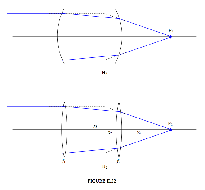
I refer now to the second part of FFigure II.22, and I suppose that the focal lengths of the two lenses are $f_1$ and $f_2$ , and the distance between them is $D$ . I now invite the reader to calculate the distances $x_2$ and $y_2$ . The distance $x_2$ can be calculated by consideration of some similar triangles (which the reader will have to add to the drawing), and the distance $y_2$ can be calculated by calculating the convergences $C_1, C_2,C_3,C_4$ in the manner which is by now familiar. You should get

$x_2 = \frac{Df_2}{f_1+f_2-D}. \label{eq:2.12.1}$

and

$y_2=\frac{f_2(f_1-D)}{f_1+f_2-D}. \label{eq:2.12.2}$

I further invite the reader to imagine that the two lenses are to be replaced by a single lens situated in the plane $H_2$ so as to bring the light to the same focus $F_2$ as was obtained by the two original lenses. The question is: what must be the focal length f of this single lens? The answer is obviously $x_2 + y_2$ , which comes to

$f = \frac{f_1f_2}{f_1+f_2-D}. \label{eq:2.12.3}$

The eyepiece of an optical instrument such as a telescope or a microscope is generally a combination of two (or more) lenses, called the field lens and the eye lens. They are generally arranged so that the distance between the two is equal to half the sum of the focal lengths of the two lenses. We shall now see that this arrangement, with two lenses made of the same glass, is relatively free from chromatic aberration.

Let us remind ourselves that the power of a lens in air is given by

$P = \frac{1}{f}=(n-1)\left(\frac{1}{r_1}+\frac{1}{r_2}\right) \label{eq:2.12.4}$

Here $r_1$ and $r_2$ are the radii of curvature of the two surfaces, and $n$ is the refractive index of the glass. For short, I am going to write Equation $\ref{eq:2.12.4}$ as

$P = \frac{1}{f} = \mu S, \label{eq:2.12.5}$

where $\mu = n-1$ and $S= \left(\frac{1}{r_1}+\frac{1}{r_2}\right)$ . That being so, Equation $\ref{eq:2.12.3}$ can be written

$P = \mu(S_1+S_2)- \mu ^2SD_1S_2 \label{eq:2.12.6}$

This equation shows how the position of the focus $F_2$ varies with colour. In particular,

$\frac{dP}{d\mu} = S_1 + S_2 - 2 \mu DS_1S_2, \label{eq:2.12.7}$

which shows that the position of $F_2$ doesn’t vary with colour provided that the distance between the lenses is

$D= \frac{S_1+S_2}{2\mu S_1S_2}. \label{eq:2.12.8}$

On going back to Equation $\ref{eq:2.12.5}$ , we see that this translates to

$\underline{\underline{D= \frac{1}{2}(f_1+f_2).}} \label{eq:2.12.9}$

Support Center

How can we help?