
4.3A: Intro Model of Thermodynamics
- Page ID
- 2563

\( \newcommand{\vecs}[1]{\overset { \scriptstyle \rightharpoonup} {\mathbf{#1}} } \)
\( \newcommand{\vecd}[1]{\overset{-\!-\!\rightharpoonup}{\vphantom{a}\smash {#1}}} \)
\( \newcommand{\dsum}{\displaystyle\sum\limits} \)
\( \newcommand{\dint}{\displaystyle\int\limits} \)
\( \newcommand{\dlim}{\displaystyle\lim\limits} \)
\( \newcommand{\id}{\mathrm{id}}\) \( \newcommand{\Span}{\mathrm{span}}\)
( \newcommand{\kernel}{\mathrm{null}\,}\) \( \newcommand{\range}{\mathrm{range}\,}\)
\( \newcommand{\RealPart}{\mathrm{Re}}\) \( \newcommand{\ImaginaryPart}{\mathrm{Im}}\)
\( \newcommand{\Argument}{\mathrm{Arg}}\) \( \newcommand{\norm}[1]{\| #1 \|}\)
\( \newcommand{\inner}[2]{\langle #1, #2 \rangle}\)
\( \newcommand{\Span}{\mathrm{span}}\)
\( \newcommand{\id}{\mathrm{id}}\)
\( \newcommand{\Span}{\mathrm{span}}\)
\( \newcommand{\kernel}{\mathrm{null}\,}\)
\( \newcommand{\range}{\mathrm{range}\,}\)
\( \newcommand{\RealPart}{\mathrm{Re}}\)
\( \newcommand{\ImaginaryPart}{\mathrm{Im}}\)
\( \newcommand{\Argument}{\mathrm{Arg}}\)
\( \newcommand{\norm}[1]{\| #1 \|}\)
\( \newcommand{\inner}[2]{\langle #1, #2 \rangle}\)
\( \newcommand{\Span}{\mathrm{span}}\) \( \newcommand{\AA}{\unicode[.8,0]{x212B}}\)
\( \newcommand{\vectorA}[1]{\vec{#1}} % arrow\)
\( \newcommand{\vectorAt}[1]{\vec{\text{#1}}} % arrow\)
\( \newcommand{\vectorB}[1]{\overset { \scriptstyle \rightharpoonup} {\mathbf{#1}} } \)
\( \newcommand{\vectorC}[1]{\textbf{#1}} \)
\( \newcommand{\vectorD}[1]{\overrightarrow{#1}} \)
\( \newcommand{\vectorDt}[1]{\overrightarrow{\text{#1}}} \)
\( \newcommand{\vectE}[1]{\overset{-\!-\!\rightharpoonup}{\vphantom{a}\smash{\mathbf {#1}}}} \)
\( \newcommand{\vecs}[1]{\overset { \scriptstyle \rightharpoonup} {\mathbf{#1}} } \)
\(\newcommand{\longvect}{\overrightarrow}\)
\( \newcommand{\vecd}[1]{\overset{-\!-\!\rightharpoonup}{\vphantom{a}\smash {#1}}} \)
\(\newcommand{\avec}{\mathbf a}\) \(\newcommand{\bvec}{\mathbf b}\) \(\newcommand{\cvec}{\mathbf c}\) \(\newcommand{\dvec}{\mathbf d}\) \(\newcommand{\dtil}{\widetilde{\mathbf d}}\) \(\newcommand{\evec}{\mathbf e}\) \(\newcommand{\fvec}{\mathbf f}\) \(\newcommand{\nvec}{\mathbf n}\) \(\newcommand{\pvec}{\mathbf p}\) \(\newcommand{\qvec}{\mathbf q}\) \(\newcommand{\svec}{\mathbf s}\) \(\newcommand{\tvec}{\mathbf t}\) \(\newcommand{\uvec}{\mathbf u}\) \(\newcommand{\vvec}{\mathbf v}\) \(\newcommand{\wvec}{\mathbf w}\) \(\newcommand{\xvec}{\mathbf x}\) \(\newcommand{\yvec}{\mathbf y}\) \(\newcommand{\zvec}{\mathbf z}\) \(\newcommand{\rvec}{\mathbf r}\) \(\newcommand{\mvec}{\mathbf m}\) \(\newcommand{\zerovec}{\mathbf 0}\) \(\newcommand{\onevec}{\mathbf 1}\) \(\newcommand{\real}{\mathbb R}\) \(\newcommand{\twovec}[2]{\left[\begin{array}{r}#1 \\ #2 \end{array}\right]}\) \(\newcommand{\ctwovec}[2]{\left[\begin{array}{c}#1 \\ #2 \end{array}\right]}\) \(\newcommand{\threevec}[3]{\left[\begin{array}{r}#1 \\ #2 \\ #3 \end{array}\right]}\) \(\newcommand{\cthreevec}[3]{\left[\begin{array}{c}#1 \\ #2 \\ #3 \end{array}\right]}\) \(\newcommand{\fourvec}[4]{\left[\begin{array}{r}#1 \\ #2 \\ #3 \\ #4 \end{array}\right]}\) \(\newcommand{\cfourvec}[4]{\left[\begin{array}{c}#1 \\ #2 \\ #3 \\ #4 \end{array}\right]}\) \(\newcommand{\fivevec}[5]{\left[\begin{array}{r}#1 \\ #2 \\ #3 \\ #4 \\ #5 \\ \end{array}\right]}\) \(\newcommand{\cfivevec}[5]{\left[\begin{array}{c}#1 \\ #2 \\ #3 \\ #4 \\ #5 \\ \end{array}\right]}\) \(\newcommand{\mattwo}[4]{\left[\begin{array}{rr}#1 \amp #2 \\ #3 \amp #4 \\ \end{array}\right]}\) \(\newcommand{\laspan}[1]{\text{Span}\{#1\}}\) \(\newcommand{\bcal}{\cal B}\) \(\newcommand{\ccal}{\cal C}\) \(\newcommand{\scal}{\cal S}\) \(\newcommand{\wcal}{\cal W}\) \(\newcommand{\ecal}{\cal E}\) \(\newcommand{\coords}[2]{\left\{#1\right\}_{#2}}\) \(\newcommand{\gray}[1]{\color{gray}{#1}}\) \(\newcommand{\lgray}[1]{\color{lightgray}{#1}}\) \(\newcommand{\rank}{\operatorname{rank}}\) \(\newcommand{\row}{\text{Row}}\) \(\newcommand{\col}{\text{Col}}\) \(\renewcommand{\row}{\text{Row}}\) \(\newcommand{\nul}{\text{Nul}}\) \(\newcommand{\var}{\text{Var}}\) \(\newcommand{\corr}{\text{corr}}\) \(\newcommand{\len}[1]{\left|#1\right|}\) \(\newcommand{\bbar}{\overline{\bvec}}\) \(\newcommand{\bhat}{\widehat{\bvec}}\) \(\newcommand{\bperp}{\bvec^\perp}\) \(\newcommand{\xhat}{\widehat{\xvec}}\) \(\newcommand{\vhat}{\widehat{\vvec}}\) \(\newcommand{\uhat}{\widehat{\uvec}}\) \(\newcommand{\what}{\widehat{\wvec}}\) \(\newcommand{\Sighat}{\widehat{\Sigma}}\) \(\newcommand{\lt}{<}\) \(\newcommand{\gt}{>}\) \(\newcommand{\amp}{&}\) \(\definecolor{fillinmathshade}{gray}{0.9}\)Construct Definitions
Work (revisited)
We introduced the expression \( W = F_{||} \Delta x \) for the work done on an object in Chapter 2, where \( F_{||} \) is the average component of the unbalanced force acting on an object parallel to the displacement of the object, \( \Delta x \). The more general expression that takes into account the fact that \( F_{||} \) can change as the object moves (i.e., \( F_{||} \) can be a function of (x)) is
\[ W = \int_{x_{i}}^{x_{f}} F(x)_{||} dx \label{workDef}\]
There are several special cases that are worth noting. First, the force can be constant. Thus, \( F(x)_{||} = F_{||} \), and \( F(x)_{||} \) can be taken outside the integral in Equation \(\ref{workDef}\) to yield our previous result:
\[ W = F_{||} \int_{x_{i}}^{x_{f}} dx = F_{||} (x_{f} - x_{i}) = F_{||} \Delta x \]
The next simplest case is when the force is a linear function of \(x\). Thus, \(F(x)_{||} = kx \), as for a spring. In this case, work then becomes
\[ W = k \int_{x_{i}}^{x_{f}} x dx = \dfrac{1}{2} k (x_{f}^{2} - x_{i}^{2})\]
Graphical Interpretation of work on an F(x) vs. x diagram
If \(F(x)\) is plotted as a function of \(x\), there is a very simple interpretation of the definite integral in the above equation: the work, \(W\), is simply the area under the \(F(x)\) curve.
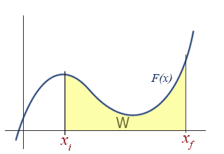
This should come as no surprise to anyone who has studied integrals. Examining the aforementioned special cases in this graphical way reveal the simplicity and utility of the graphical approach.
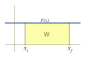
Work Due To a Constant Force
The graph of a constant function is a horizontal line. The region under a line is a rectangle, who's area is simply \( F \Delta x \).
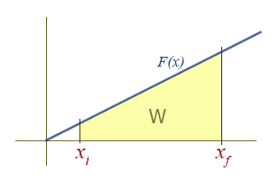
Work Due To a Linear Force as a Function of Position
This is how springs and sometimes pendulums are treated, and is the basis for the simple harmonic oscillator, a widely applicable model. To find the work done graphically, we must compute the area of the yellow region, which in this case is a trapezoid. There is an area formula for a trapezoid, which is \( A = \dfrac{h_1 + h_2}{2} b \). However, it might be more intuitive to see it as a difference of two triangles in this case: A large triangle with its tip missing, or \( \dfrac{1}{2}b_{2}h_{2} - \dfrac{1}{2}b_{1}h_{1} \).
To retrieve the more familiar \( \dfrac{1}{2} k (x_{f}^{2} - x_{i}^{2}) \), remember that the function is of the form \( F(x)_{||} = kx \), and the height \( h \) of the triangle is the value of \( F(x)_{||} \). Then,
since the base of the triangle \(b\) is just the x coordinate of the right side of the triangle, we have
\[ W = \dfrac{1}{2}b_{2}h_{2} - \dfrac{1}{2}b_{1}h_{1} = \dfrac{1}{2}(x_{f})(kx_{f}) - \dfrac{1}{2}(x_{i})(kx_{i}) \]
\[ = \dfrac{1}{2} k (x_{f}^{2} - x_{i}^{2})\]
Differential Expression:
Rather than the integral expression for work, it is often convenient to use a differential expression. That is, we want to talk about the small increment of work corresponding to the product of the parallel component of force and the differential increment of distance, dx.
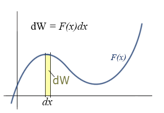
This expression for the incremental work fits nicely with the graphical representation of work and the graphical interpretation of the definite integral. If you do not remember this from your calculus class, you might want to go back and review it over the next couple of weeks. (The graphical interpretations of derivatives and integrals are two of the those important concepts that you should take away from calculus, i.e., things you remember for the rest of your life.)
Work Done on a Fluid
We now have general expressions for work in terms of forces and distances moved. But when you push on a fluid (i.e., a liquid or a gas), the magnitude of the force depends on how hard you push as well as the area of your hand. It depends on a property of the fluid–a property we call pressure. Pressure turns out to be an important and useful property of a fluid. It has to do with how much the fluid is “squeezed”. The force exerted on a fluid by an object of cross-sectional area A is proportional to the pressure P and area A and is directed in a direction perpendicular to A.
The force pushing the movable piston to the right is equal (when there are no accelerations) to the force the fluid contained in the cylinder exerts on the piston to the left. The magnitude of this force is not a definition of pressure, but simply the relation of force to pressure.
\[ P = \dfrac{F}{A} \]
The dimensionality of pressure is force per area, which is also energy per volume:
\[ \text{Pressure} = \dfrac{\text{Force}}{ \text{length}^2} = \dfrac{\text{Energy}}{ \text{length}^3} = \dfrac{\text{Energy}}{\text{volume}}\]
Useful reference information
The units of pressure in SI are the Pascal (Pa):
\[ \text{Pressure} = \dfrac{N}{m^{2}} = \dfrac{J}{m^{3}} = \text{[Pascal]}\]
Some useful conversions involving pressure are
\(1.0 atm = 1.01 \times 10^{5} Pa = 14.7 lb/in^{2} (psi) \)
Our previous expressions for work were in terms of the linear distance -- a product of force and displacement. However, when dealing with fluids, it is useful to make a change of variables from \(x\) to \(V\). For the case of a piston, the relation between the differentials \(dV\) and \(dx\) is illustrated in the figure.
Note: The reason for the minus sign in front of dV is because the volume gets smaller as “x” increases.
To extend the definition of work to fluids using \(V\) and \(dV\) rather than \(x\) and \(dx\), use \( dV = -Adx \) to make the change of variables.
\[ W = \int_{x_{i}}^{x_{f}} F(x)_{||} dx \]
Substitute \(\dfrac{-dV}{A}\) for \(dx\) and use the relationship between force, pressure and area to substitute \(F(x)_{||} \) for \(P(V) A \), and the integral becomes:
\[ W = - \int_{v_{i}}^{v_{f}} P(V)A \cdot \dfrac{dV}{A} = - \int_{v_{i}}^{v_{f}} P(V) dV \]
This is the expression for the work done on a fluid when it is compressed from a volume Vi to a volume Vf. Note that the minus sign in front of the integral ensures that work comes out positive (since \(PdV\) is negative). If instead of being compressed, the volume expands, the work done on the fluid will be negative. Equivalently, we can say that the fluid does positive work on some other physical system.
In differential form, the work done when changing the volume of a fluid is:
\[dW = -P(V) dV \]
To proceed further, we need to know how the pressure, \(P\), depends on the volume, \(V\). For gases that are not too dense, we can use the ideal gas law, which relates the volume, pressure, temperature T, and number of gas particles N (or number of moles n):
Ideal Gas Law
An important relationship between the pressure, temperature, volume, and number of particles in an ideal gas. This is an extremely useful equation, and is worth remembering. It's also important to remember that it is only true under the conditions where intermolecular interactions are negligible.
\[ P V = N k_B T\]
or
\[P V = n R T \]
where \(k_B\) is Boltzmann’s constant and \(R\) is the gas constant familiar from chemistry. In addition, \(n\) is the number of moles, while \(N\) is the actual number of molecules.
\[n = \dfrac{N}{N_A}\]
where \(N_a\) is Avogadro's constrant (\(6.022 \times 10^{23}\)). Note that
\[k_B = \dfrac{R}{N_A} =1.381 \times 10^{-23}\; J/K\]
and
\[R = 8.314 \,J / mol \cdot K\]
The ideal gas law states that pressure and volume are not uniquely related, but depend on the temperature. Therefore, the work done when compressing a gas will depend on how temperature changes as the pressure and volume change. That is, it takes different amounts of work to compress a gas, depending on how the temperature varies during the compression, as heat is or is not allowed to enter the system. PV diagrams and a new way of stating conservation of energy will allow us to determine the contributions of work and heat to changes in systems.
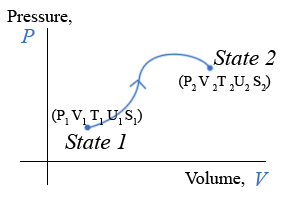
State of a Physical System, Equilibrium State
One aspect of thermodynamics that we will pursue is how systems evolve from one state to another. To understand this we need to be able to describe the initial and final endpoint states and to describe the process for getting from one to the other. In describing individual states, we can use certain variables that have unique values for any state. These variables are called “state variables.” For example, an ideal gas in a particular state will have one value for P, V, T, and U. Relationships between these variables are expressed in “equations of state.” You are already familiar (from chemistry) with one equation of state – the ideal gas equation (PV = nRT). As a system changes, due to heat or work being added or removed, the values of these state variables will change.
Previously we found it was useful to use energy-system diagrams to help us focus on changes of energy. These energy-system diagrams were a useful representational tool. To describe changes in state variables as a system undergoes change, we can use a different representational tool: state diagrams. A state diagram is a graph of one state variable plotted as a function of another state variable for a particular process. Because it is frequently the case that two state variables completely determine the “state” of the system, a two dimensional state diagram can be a very useful representational tool. Often, the pressure, P, and volume, V, are chosen to be the two state variables. Another useful pair is entropy and temperature.
State Diagrams
One reason the two-variable state diagram is such a useful representation, is because it is possible to easily follow the path a system takes as it undergoes the process for going from the initial to the final state. By path, we mean the continuous line of intermediate states that a system passes through, as it moves from an initial to a final state. The PV diagram below shows one of the infinite number of possible paths connecting state-1 with state-2.
Equilibrium State
It makes no sense to try to represent a state of a system on state diagram, unless the system is in equilibrium. The state variables, which are macroscopic variables, must have unique values that are the same throughout the system. Likewise, it makes no sense to talk about a particular path along a state diagram unless all the intermediate states are equilibrium states as well. This is not to say that a real physical system can’t go from one state, say state-1 in the example above to state 2 and not follow a set of intermediate states that are equilibrium states. In fact, most processes do not follow a path that continuously moves along a set of equilibrium states. It is just that we can’t show the path if it does not pass through a series of equilibrium states. The end points, however, are well defined, regardless of how the system gets from the initial to the final equilibrium state. The system can start in an equilibrium state and end up in an equilibrium state and never be in an equilibrium state along the way.
PV Diagram
We will find many uses for PV-diagrams in connection with understanding the energy exchanges that take place as thermodynamic systems undergo change. One of the most important things we have already seen is that the area under a PV-curve represents the work done on or by the system during a volume change. This work, in turn, is directly related to heat transfer and changes in the internal energy of the system.
Heat Capacity at Constant V and at Constant P
Any heat capacity measurement consists of adding a known amount of heat to a substance and measuring the temperature change.
\[ C = \frac{dQ}{dT} \]
For now, we consider only substances whose only internal energies are bond and thermal and we specifically make the heat capacity measurement at temperatures where bond energy changes do NOT occur. But there is still an issue as to whether the system we are interested does work (or has work done on it) during the process of adding heat to make the heat capacity measurement. Consequently, it is common to define to specific processes: one at constant volume, so that no work is done, and the other at constant pressure, so, especially with gases, there is definitely work involved. We will come back to this shortly at the end of the discussion on relationships between the constructs.
A New State Function: Enthalpy, H
A state function depends only on the condition of a system at a particular time. It does not depend on how it got to be in that condition. The state function we have been dealing with all quarter is, of course, energy. The energy of a system depends only on the values of some state variables at the particular time. Work and heat are not state variables. They are processes. Their values depend on how a system is changed. This distinction is critically important to understand.
If you look up values of most thermal properties such as heats of fusion, vaporization, or combustion, you will often find them tabulated as changes of enthalpy, expressed by the symbol ∆H. Enthalpy, like energy, is a state function. It depends only on the values of certain parameters at that time, but does not depend on how the system got to those values. We will see how this comes about in the relationship section shortly.
Another New State Function: Entropy, S
We will also take a close look at another state function, the entropy, S. Entropy is directly connected to the statistical behavior of large numbers of particles. In addition to using the statistical approach, we will examine entropy from the perspective of thermodynamics, to see how it is related to other thermodynamic variables. Using both approaches will help us to make better sense out of what is often a very confusing and mysterious concept.
Reversible Process or Reversible Path
One way to think about reversibility is simply to ask, can a system move along a path and then stop and have the process “run backwards” and get back to exactly the same state by following along the exact same path? For this to happen two conditions have to be met. First, there can be no friction. Friction causes energy to be transferred to thermal energy systems, which can never be completely “gotten back out” of thermal systems into mechanical systems. Second, there can be no heat transfers across finite temperature differences. This last statement is a little hard to handle. The only way to have heat transfers is to have temperature differences. One way to think about this is to say to yourself, “Well, I will create just a little bitty temperature difference and wait a long time for the heat to transfer, but there will never be very much of a temperature difference.” If you have enough patience, you can make it almost reversible. So in real life, there are no truly reversible processes, but it is possible to come fairly close. And, you can certainly calculate along reversible paths, which is the real reason for this distinction.
Contributors
Authors of Phys7A (UC Davis Physics Department)