Basal Metabolism
- Page ID
- 3350
\( \newcommand{\vecs}[1]{\overset { \scriptstyle \rightharpoonup} {\mathbf{#1}} } \)
\( \newcommand{\vecd}[1]{\overset{-\!-\!\rightharpoonup}{\vphantom{a}\smash {#1}}} \)
\( \newcommand{\dsum}{\displaystyle\sum\limits} \)
\( \newcommand{\dint}{\displaystyle\int\limits} \)
\( \newcommand{\dlim}{\displaystyle\lim\limits} \)
\( \newcommand{\id}{\mathrm{id}}\) \( \newcommand{\Span}{\mathrm{span}}\)
( \newcommand{\kernel}{\mathrm{null}\,}\) \( \newcommand{\range}{\mathrm{range}\,}\)
\( \newcommand{\RealPart}{\mathrm{Re}}\) \( \newcommand{\ImaginaryPart}{\mathrm{Im}}\)
\( \newcommand{\Argument}{\mathrm{Arg}}\) \( \newcommand{\norm}[1]{\| #1 \|}\)
\( \newcommand{\inner}[2]{\langle #1, #2 \rangle}\)
\( \newcommand{\Span}{\mathrm{span}}\)
\( \newcommand{\id}{\mathrm{id}}\)
\( \newcommand{\Span}{\mathrm{span}}\)
\( \newcommand{\kernel}{\mathrm{null}\,}\)
\( \newcommand{\range}{\mathrm{range}\,}\)
\( \newcommand{\RealPart}{\mathrm{Re}}\)
\( \newcommand{\ImaginaryPart}{\mathrm{Im}}\)
\( \newcommand{\Argument}{\mathrm{Arg}}\)
\( \newcommand{\norm}[1]{\| #1 \|}\)
\( \newcommand{\inner}[2]{\langle #1, #2 \rangle}\)
\( \newcommand{\Span}{\mathrm{span}}\) \( \newcommand{\AA}{\unicode[.8,0]{x212B}}\)
\( \newcommand{\vectorA}[1]{\vec{#1}} % arrow\)
\( \newcommand{\vectorAt}[1]{\vec{\text{#1}}} % arrow\)
\( \newcommand{\vectorB}[1]{\overset { \scriptstyle \rightharpoonup} {\mathbf{#1}} } \)
\( \newcommand{\vectorC}[1]{\textbf{#1}} \)
\( \newcommand{\vectorD}[1]{\overrightarrow{#1}} \)
\( \newcommand{\vectorDt}[1]{\overrightarrow{\text{#1}}} \)
\( \newcommand{\vectE}[1]{\overset{-\!-\!\rightharpoonup}{\vphantom{a}\smash{\mathbf {#1}}}} \)
\( \newcommand{\vecs}[1]{\overset { \scriptstyle \rightharpoonup} {\mathbf{#1}} } \)
\(\newcommand{\longvect}{\overrightarrow}\)
\( \newcommand{\vecd}[1]{\overset{-\!-\!\rightharpoonup}{\vphantom{a}\smash {#1}}} \)
\(\newcommand{\avec}{\mathbf a}\) \(\newcommand{\bvec}{\mathbf b}\) \(\newcommand{\cvec}{\mathbf c}\) \(\newcommand{\dvec}{\mathbf d}\) \(\newcommand{\dtil}{\widetilde{\mathbf d}}\) \(\newcommand{\evec}{\mathbf e}\) \(\newcommand{\fvec}{\mathbf f}\) \(\newcommand{\nvec}{\mathbf n}\) \(\newcommand{\pvec}{\mathbf p}\) \(\newcommand{\qvec}{\mathbf q}\) \(\newcommand{\svec}{\mathbf s}\) \(\newcommand{\tvec}{\mathbf t}\) \(\newcommand{\uvec}{\mathbf u}\) \(\newcommand{\vvec}{\mathbf v}\) \(\newcommand{\wvec}{\mathbf w}\) \(\newcommand{\xvec}{\mathbf x}\) \(\newcommand{\yvec}{\mathbf y}\) \(\newcommand{\zvec}{\mathbf z}\) \(\newcommand{\rvec}{\mathbf r}\) \(\newcommand{\mvec}{\mathbf m}\) \(\newcommand{\zerovec}{\mathbf 0}\) \(\newcommand{\onevec}{\mathbf 1}\) \(\newcommand{\real}{\mathbb R}\) \(\newcommand{\twovec}[2]{\left[\begin{array}{r}#1 \\ #2 \end{array}\right]}\) \(\newcommand{\ctwovec}[2]{\left[\begin{array}{c}#1 \\ #2 \end{array}\right]}\) \(\newcommand{\threevec}[3]{\left[\begin{array}{r}#1 \\ #2 \\ #3 \end{array}\right]}\) \(\newcommand{\cthreevec}[3]{\left[\begin{array}{c}#1 \\ #2 \\ #3 \end{array}\right]}\) \(\newcommand{\fourvec}[4]{\left[\begin{array}{r}#1 \\ #2 \\ #3 \\ #4 \end{array}\right]}\) \(\newcommand{\cfourvec}[4]{\left[\begin{array}{c}#1 \\ #2 \\ #3 \\ #4 \end{array}\right]}\) \(\newcommand{\fivevec}[5]{\left[\begin{array}{r}#1 \\ #2 \\ #3 \\ #4 \\ #5 \\ \end{array}\right]}\) \(\newcommand{\cfivevec}[5]{\left[\begin{array}{c}#1 \\ #2 \\ #3 \\ #4 \\ #5 \\ \end{array}\right]}\) \(\newcommand{\mattwo}[4]{\left[\begin{array}{rr}#1 \amp #2 \\ #3 \amp #4 \\ \end{array}\right]}\) \(\newcommand{\laspan}[1]{\text{Span}\{#1\}}\) \(\newcommand{\bcal}{\cal B}\) \(\newcommand{\ccal}{\cal C}\) \(\newcommand{\scal}{\cal S}\) \(\newcommand{\wcal}{\cal W}\) \(\newcommand{\ecal}{\cal E}\) \(\newcommand{\coords}[2]{\left\{#1\right\}_{#2}}\) \(\newcommand{\gray}[1]{\color{gray}{#1}}\) \(\newcommand{\lgray}[1]{\color{lightgray}{#1}}\) \(\newcommand{\rank}{\operatorname{rank}}\) \(\newcommand{\row}{\text{Row}}\) \(\newcommand{\col}{\text{Col}}\) \(\renewcommand{\row}{\text{Row}}\) \(\newcommand{\nul}{\text{Nul}}\) \(\newcommand{\var}{\text{Var}}\) \(\newcommand{\corr}{\text{corr}}\) \(\newcommand{\len}[1]{\left|#1\right|}\) \(\newcommand{\bbar}{\overline{\bvec}}\) \(\newcommand{\bhat}{\widehat{\bvec}}\) \(\newcommand{\bperp}{\bvec^\perp}\) \(\newcommand{\xhat}{\widehat{\xvec}}\) \(\newcommand{\vhat}{\widehat{\vvec}}\) \(\newcommand{\uhat}{\widehat{\uvec}}\) \(\newcommand{\what}{\widehat{\wvec}}\) \(\newcommand{\Sighat}{\widehat{\Sigma}}\) \(\newcommand{\lt}{<}\) \(\newcommand{\gt}{>}\) \(\newcommand{\amp}{&}\) \(\definecolor{fillinmathshade}{gray}{0.9}\)Basal Metabolic Rate
This document discusses the metabolic rate of different animals, and how it scales with the mass of the creature. It was originally written as a Supplementary Topic for a first year course at the University of Toronto: Physics for the Life Sciences I.
Metabolism
Our bodies produce energy from the food that we eat. The rate at which this energy is produced by our metabolism is called the metabolic rate, and is often measured in watts. Other common units include kcal/day. The basal metabolic rate (BMR) is the metabolic rate when the organism is resting. The table shows some basal metabolic rates for various animals. It can be seen that as the mass increases so does the BMR.
| Animal | Mass (kg) | Basal Metabolic Rate (watts) |
|---|---|---|
|
Dove
|
0.16
|
0.97
|
|
Rat
|
0.26
|
1.45
|
|
Pigeon
|
0.30
|
1.55
|
|
Hen
|
2.0
|
4.8
|
|
Dog (female)
|
11
|
14.5
|
|
Dog (male)
|
16
|
20
|
|
Sheep
|
45
|
50
|
|
Woman
|
60
|
68
|
|
Man
|
70
|
87
|
|
Cow
|
400
|
266
|
|
Steer
|
680
|
411
|
These numbers are "generic" in the sense that there are large variations among individuals.
Sadly, as is common for biological data taken or compiled by people who have not taken the PHY138 laboratory at U of T or another good course in data analysis, there are no errors given with the above numbers. We see that for people, then, when resting we are generating energy at a rate equal to a typical incandescent light bulb. If we are being physically active, our metabolic rate increases and the extra energy is used for the activity. Rates of 400 W or more are common for physically fit athletes.
Heat Radiation
Consider a resting woman whose metabolism is generating 68 watts, almost the same power as a 60 watt incandescent light bulb. If her body is radiating energy into the room at a rate of 68 watts, then she is in thermal equilibrium. If her metabolic rate remains constant and she begins to radiate thermal energy into her environment at a greater rate that 68 W she will get cold.
Now, the rate at which heat energy is radiated from an object is proportional to the difference in temperature between the surface of the object and the temperature of the surroundings. This is usually called Newton's Law of Cooling.
This means that if we are in a cold room we radiate away energy faster than in a warm room, and start feeling cold. The body will begin to shiver, which increases the metabolic rate. Metabolic rates of 200 W or more are possible for people who are shivering.
Julius Robert Mayer was a German-born physician. In the early 1800's he noticed that people who lived in Indonesia had blood which was a deeper red than people living in Europe. This indicated that they had less oxygen in their blood, which meant their metabolic rate was lower than Europeans. He reasoned that this was because to maintain equilibrium with their warmer environment required a lower metabolic rate. This was one of the very first realizations the heat is just another form of energy. Mayer's first paper on this realization was rejected, largely because he was a physician and largely ignorant about physics. Although disappointed, Mayer took up the study of physics, learned about kinetic energy, and his second paper was published in 1842.
Note: Mayer did not use the vocabulary of the previous paragraph in his reasoning.
There is another factor that relates to the radiation of heat energy, the surface area A of the body doing the radiating. In terms of the power, i.e. energy per time:
\[\frac{dE}{dt}=kA\label{1}\]
Here k is a constant. This relation explains why, for example, air cooled motorcycle engines have fins: this greatly increases the effective surface area so the engine radiates heat at a much faster rate.
Dimensional Analysis
Imagine we have 2 objects with the same shape but different sizes.We characterise the size of the object by some length L. For a sphere L might be the radius or diameter, for a cube it might be the length of one of the sides, for an elephant it might be the height. Regardless of the choice for how we characterise the size of the objects, the surface area scales as:
\[A \propto L^2 \label{2}\]
For different species of animals, we might expect this scaling to also be approximately true, although the effective surface area of, for example, an animal with fur is greater than the effective surface area of an animal of the same size but with no fur.
For an object with density \(\rho\) and volume V the mass m is:
\[m=\rho V \label{3}\]
For different objects characterised by some length L the volume scales as:
\[V\propto L^3 \label{4}\]
Since, from Eqn (3), the mass is proportional to the volume, it is proportional to the length to the third power:
\[m\propto L^3 \label{5}\]
We can state this same relation by saying that the length is proportional to the cube root of the mass:
\[L\propto m^{\frac{1}{3}} \label{6}\]
Then the square of L scales as the mass m to the two-thirds power:
\[L^2\propto m^{\frac{2}{3}} \label{7}\]
We saw in Eqn (2) that the surface area scales as the square of L, so in terms of the mass:
\[A\propto L^2 \propto m^{\frac{2}{3}}\label{9} \]
In the previous section we saw that the rate at which an organism gives up heat to its surroundings is proportional to the area, Eqn (1), so we now see that it is proportional to the mass to the two-thirds power:
\[\frac{dE}{dt}=cm^{\frac{2}{3}}\label{10}\]
where c is a constant.
But, we have seen that at equilibrium the rate at which the organism radiates energy is proportional to its metabolic rate. Therefore we predict that the basal metabolic rate of different organisms should scale as the two-thirds power of their mass.
\[bmr=cm^{\frac{2}{3}}\label{11}\]
This type of dimensional analysis leading to Eqn (11) is often called allometry.
Data Analysis
Experimentally, to investigate the validity of Eqn (11), it is convenient to take the logarithm of both sides:
\[\ln(bmr)=\ln(c)+\frac{2}{3} \ln(m) \label{12}\]
Then we can fit the logarithm of the basal metabolic rate versus the logarithm of the mass to a straight line. The intercept of the result of the fit is ln(c) and the slope should be two-thirds.
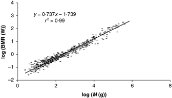
However, as first determined by Kleiber in 1932, the result of the fit gives a slope of almost exactly 3/4.
The figure is a recent compilation of data for mammals.
Source: V. M. Savage, J. F. Gillooly, W. H. Woodruff, G. B. West, A. P. Allen, B. J. Enquist, J. H. Brown, "The predominance of quarter-power scaling in biology", Jour. Functional Ecology 18, (2004) 257-282.
So experimentally Eqn (11) is not correct. Instead:
\[bmr=cm^{\frac{3}{4}}\label{13}\]
Eqn (13) is called Kleiber's Law, and has been shown to be approximately true over 27 orders of magnitude in the value of the mass, from the terminal oxidize molecules of the respiratory complex to whales!
Other relationships involving living organisms show similar scaling as the three-quarter power of the total mass of the organism. Examples include brain mass. Other properties scale as the one-quarter or one-half power of the mass; examples include the heart rate (-1/4), lifespan (1/4), unicellular genome lengths (1/4), and RNA concentration (-1/4).
The fact that heart rate goes down as the body mass to the -1/4 power while lifespan goes up as the body mass to the +1/4 power means that the number of heart beats in a lifetime is roughly constant independent of the kind animal.
Why?
Various attempts to explain these facts have been made. One particularly interesting approach is by West, Brown and Enquist in 1997. West is a High Energy physicist, and Brown and Enquist are ecologists.
|
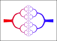
The figure to the right is a representation of the circulatory system. It shows how the arteries, in red, branch into smaller arteries, and finally into the capillaries; the capillaries then coalesce into small veins, in blue, which in turn coalesce into still larger veins. The original source of the figure is |
 |
West, Brown and Enquist realised that the above figure is very similar to a fractal, which you may know are objects with non-integer, i.e. fractional, dimensions. A very brief introduction to fractals is available here.
In their analysis, then, the metabolism scales as the dimension of the circulatory system, which is after all what delivers the energy being metabolized. The result of their calculations is Kleiber's Law: the BMR scales as the three-quarter power of the mass.


