
1.10.3: Electromagnetic transverse waves
- Page ID
- 128482
\( \newcommand{\vecs}[1]{\overset { \scriptstyle \rightharpoonup} {\mathbf{#1}} } \)
\( \newcommand{\vecd}[1]{\overset{-\!-\!\rightharpoonup}{\vphantom{a}\smash {#1}}} \)
\( \newcommand{\dsum}{\displaystyle\sum\limits} \)
\( \newcommand{\dint}{\displaystyle\int\limits} \)
\( \newcommand{\dlim}{\displaystyle\lim\limits} \)
\( \newcommand{\id}{\mathrm{id}}\) \( \newcommand{\Span}{\mathrm{span}}\)
( \newcommand{\kernel}{\mathrm{null}\,}\) \( \newcommand{\range}{\mathrm{range}\,}\)
\( \newcommand{\RealPart}{\mathrm{Re}}\) \( \newcommand{\ImaginaryPart}{\mathrm{Im}}\)
\( \newcommand{\Argument}{\mathrm{Arg}}\) \( \newcommand{\norm}[1]{\| #1 \|}\)
\( \newcommand{\inner}[2]{\langle #1, #2 \rangle}\)
\( \newcommand{\Span}{\mathrm{span}}\)
\( \newcommand{\id}{\mathrm{id}}\)
\( \newcommand{\Span}{\mathrm{span}}\)
\( \newcommand{\kernel}{\mathrm{null}\,}\)
\( \newcommand{\range}{\mathrm{range}\,}\)
\( \newcommand{\RealPart}{\mathrm{Re}}\)
\( \newcommand{\ImaginaryPart}{\mathrm{Im}}\)
\( \newcommand{\Argument}{\mathrm{Arg}}\)
\( \newcommand{\norm}[1]{\| #1 \|}\)
\( \newcommand{\inner}[2]{\langle #1, #2 \rangle}\)
\( \newcommand{\Span}{\mathrm{span}}\) \( \newcommand{\AA}{\unicode[.8,0]{x212B}}\)
\( \newcommand{\vectorA}[1]{\vec{#1}} % arrow\)
\( \newcommand{\vectorAt}[1]{\vec{\text{#1}}} % arrow\)
\( \newcommand{\vectorB}[1]{\overset { \scriptstyle \rightharpoonup} {\mathbf{#1}} } \)
\( \newcommand{\vectorC}[1]{\textbf{#1}} \)
\( \newcommand{\vectorD}[1]{\overrightarrow{#1}} \)
\( \newcommand{\vectorDt}[1]{\overrightarrow{\text{#1}}} \)
\( \newcommand{\vectE}[1]{\overset{-\!-\!\rightharpoonup}{\vphantom{a}\smash{\mathbf {#1}}}} \)
\( \newcommand{\vecs}[1]{\overset { \scriptstyle \rightharpoonup} {\mathbf{#1}} } \)
\(\newcommand{\longvect}{\overrightarrow}\)
\( \newcommand{\vecd}[1]{\overset{-\!-\!\rightharpoonup}{\vphantom{a}\smash {#1}}} \)
\(\newcommand{\avec}{\mathbf a}\) \(\newcommand{\bvec}{\mathbf b}\) \(\newcommand{\cvec}{\mathbf c}\) \(\newcommand{\dvec}{\mathbf d}\) \(\newcommand{\dtil}{\widetilde{\mathbf d}}\) \(\newcommand{\evec}{\mathbf e}\) \(\newcommand{\fvec}{\mathbf f}\) \(\newcommand{\nvec}{\mathbf n}\) \(\newcommand{\pvec}{\mathbf p}\) \(\newcommand{\qvec}{\mathbf q}\) \(\newcommand{\svec}{\mathbf s}\) \(\newcommand{\tvec}{\mathbf t}\) \(\newcommand{\uvec}{\mathbf u}\) \(\newcommand{\vvec}{\mathbf v}\) \(\newcommand{\wvec}{\mathbf w}\) \(\newcommand{\xvec}{\mathbf x}\) \(\newcommand{\yvec}{\mathbf y}\) \(\newcommand{\zvec}{\mathbf z}\) \(\newcommand{\rvec}{\mathbf r}\) \(\newcommand{\mvec}{\mathbf m}\) \(\newcommand{\zerovec}{\mathbf 0}\) \(\newcommand{\onevec}{\mathbf 1}\) \(\newcommand{\real}{\mathbb R}\) \(\newcommand{\twovec}[2]{\left[\begin{array}{r}#1 \\ #2 \end{array}\right]}\) \(\newcommand{\ctwovec}[2]{\left[\begin{array}{c}#1 \\ #2 \end{array}\right]}\) \(\newcommand{\threevec}[3]{\left[\begin{array}{r}#1 \\ #2 \\ #3 \end{array}\right]}\) \(\newcommand{\cthreevec}[3]{\left[\begin{array}{c}#1 \\ #2 \\ #3 \end{array}\right]}\) \(\newcommand{\fourvec}[4]{\left[\begin{array}{r}#1 \\ #2 \\ #3 \\ #4 \end{array}\right]}\) \(\newcommand{\cfourvec}[4]{\left[\begin{array}{c}#1 \\ #2 \\ #3 \\ #4 \end{array}\right]}\) \(\newcommand{\fivevec}[5]{\left[\begin{array}{r}#1 \\ #2 \\ #3 \\ #4 \\ #5 \\ \end{array}\right]}\) \(\newcommand{\cfivevec}[5]{\left[\begin{array}{c}#1 \\ #2 \\ #3 \\ #4 \\ #5 \\ \end{array}\right]}\) \(\newcommand{\mattwo}[4]{\left[\begin{array}{rr}#1 \amp #2 \\ #3 \amp #4 \\ \end{array}\right]}\) \(\newcommand{\laspan}[1]{\text{Span}\{#1\}}\) \(\newcommand{\bcal}{\cal B}\) \(\newcommand{\ccal}{\cal C}\) \(\newcommand{\scal}{\cal S}\) \(\newcommand{\wcal}{\cal W}\) \(\newcommand{\ecal}{\cal E}\) \(\newcommand{\coords}[2]{\left\{#1\right\}_{#2}}\) \(\newcommand{\gray}[1]{\color{gray}{#1}}\) \(\newcommand{\lgray}[1]{\color{lightgray}{#1}}\) \(\newcommand{\rank}{\operatorname{rank}}\) \(\newcommand{\row}{\text{Row}}\) \(\newcommand{\col}{\text{Col}}\) \(\renewcommand{\row}{\text{Row}}\) \(\newcommand{\nul}{\text{Nul}}\) \(\newcommand{\var}{\text{Var}}\) \(\newcommand{\corr}{\text{corr}}\) \(\newcommand{\len}[1]{\left|#1\right|}\) \(\newcommand{\bbar}{\overline{\bvec}}\) \(\newcommand{\bhat}{\widehat{\bvec}}\) \(\newcommand{\bperp}{\bvec^\perp}\) \(\newcommand{\xhat}{\widehat{\xvec}}\) \(\newcommand{\vhat}{\widehat{\vvec}}\) \(\newcommand{\uhat}{\widehat{\uvec}}\) \(\newcommand{\what}{\widehat{\wvec}}\) \(\newcommand{\Sighat}{\widehat{\Sigma}}\) \(\newcommand{\lt}{<}\) \(\newcommand{\gt}{>}\) \(\newcommand{\amp}{&}\) \(\definecolor{fillinmathshade}{gray}{0.9}\)Transverse electric and magnetic fields produce each other in light, radio waves and other electromagnetic radiation. Here we demonstrate that electromagnetic radiation is a transverse rather than a longitudinal wave. This page supports the multimedia tutorial The Nature of Light.
- The electric field direction and the direction of propagation
- Electric and magnetic fields
- Polarised light
The electric field direction and the direction of propagationIs light and other electromagnetic radiation longitudinal (like sound) or transverse (like waves in a rope)? Here we transmit and receive UHF radio waves to find out.
A horizontal dipole antenna transmits radiation with an electric field parallel to the dipole axis: i.e. horizontal. In the first experiment, I rotate a receiving antenna in the vertical plane. This dipole antenna is connected to the oscilloscope whose screen we see at left. The signal is maximal when the antenna is horizontal and smallest when vertical. So, in this plane, the strongest signal is in the horizontal direction. In the next experiment, I rotate the receiving antenna in a plane that is nearly horizontal: it is the plane including the line from the camera to the transmitter and a horizontal line at right angles to this.
The signal is maximal when the antenna is smallest when it lies in the line pointing to and largest when at right angles to that line. So, in this plane, the strongest signal is at right angles to the direction of propagation. So the electric field is in the direction at right angles to that of propagation. The magnetic field generated by a current in a wire, as in the transmitting antenna, forms circles around it. So the magnetic field is at right angles to both the electric field and the direction of propagation.
|
||||
Electric and magnetic fieldsThe animation below shows the electric field E and magnetic field B in one-dimensional propagation.
In Maxwell's equations, the spatial variation in E is related to the time variation in B and vice versa. This gives rise to a wave solution, with speed c. Maxwell used the equality of speed of light and electromagnetic radiation to argue that light was electromagnetic. |
||||
Polarised lightIn light, the plane including the direction of propagation and the direction of the electric field is called the plane of polarisation. In totally polarised light, all photons have the same plane of polarisation. In unpolarised light, photons are present with polarisations in all planes including the direction of propagation.
Light reflected from horizontal surfaces often has significant polarisation in the horizontal direction. The 'glare' reflected from horizontal surfaces can therefore be reduced with sunglasses that admit only light with vertical polarisation. Here we show what happens when light is passed through one polarising filter (one pair of such glasses) and then through another, whose relative orientation is changed. The following link returns you to the multimedia tutorial The Nature of Light |


Transverse waves propagate through media with a speed orthogonally to the direction of energy transfer.
learning objectives
- Describe properties of the transverse wave
A transverse wave is a moving wave that consists of oscillations occurring perpendicular (or right angled) to the direction of energy transfer. If a transverse wave is moving in the positive x-direction, its oscillations are in up and down directions that lie in the y–z plane. Light is an example of a transverse wave. For transverse waves in matter, the displacement of the medium is perpendicular to the direction of propagation of the wave. A ripple on a pond and a wave on a string are easily visualized transverse waves.
Transverse waves are waves that are oscillating perpendicularly to the direction of propagation. If you anchor one end of a ribbon or string and hold the other end in your hand, you can create transverse waves by moving your hand up and down. Notice though, that you can also launch waves by moving your hand side-to-side. This is an important point. There are two independent directions in which wave motion can occur. In this case, these are the y and z directions mentioned above. depicts the motion of a transverse wave. Here we observe that the wave is moving in t and oscillating in the x-y plane. A wave can be thought as comprising many particles (as seen in the figure) which oscillate up and down. In the figure we observe this motion to be in x-y plane (denoted by the red line in the figure). As time passes the oscillations are separated by units of time. The result of this separation is the sine curve we expect when we plot position versus time.
Figure \(\PageIndex{1}\): Sine Wave: The direction of propagation of this wave is along the t axis. (Copyright: CC0 Nashev at Wikipedia)
When a wave travels through a medium–i.e., air, water, etc., or the standard reference medium (vacuum)–it does so at a given speed: this is called the speed of propagation. The speed at which the wave propagates is denoted and can be found using the following formula:
\[\mathrm{v=fλ}\]
where v is the speed of the wave, f is the frequency , and is the wavelength. The wavelength spans crest to crest while the amplitude is 1/2 the total distance from crest to trough. Transverse waves have their applications in many areas of physics. Examples of transverse waves include seismic S (secondary) waves, and the motion of the electric (E) and magnetic (M) fields in an electromagnetic plane waves, which both oscillate perpendicularly to each other as well as to the direction of energy transfer. Therefore an electromagnetic wave consists of two transverse waves, visible light being an example of an electromagnetic wave.
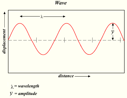
Figure \(\PageIndex{2}\): Wavelength and Amplitude: The wavelength is the distance between adjacent crests. The amplitude is the 1/2 the distance from crest to trough. (Copyright: Roger B and Oleg Alexandrov GNU Free Document License at Wikipedia
Wavelength and Amplitude: The wavelength is the distance between adjacent crests. The amplitude is the 1/2 the distance from crest to trough.
Two Types of Waves: Longitudinal vs. Transverse: Even ocean waves!
We find that electromagnetic waves carry energy. Electromagnetic radiation (EMR) carries energy—sometimes called radiant energy—through space continuously away wfrom the source (this is not true of the near-field part of the EM field). Electromagnetic waves can be imagined as a self-propagating transverse oscillating wave of electric and magnetic fields. EMR also carries both momentum and angular momentum. These properties may all be imparted to matter with which it interacts (through work). EMR is produced from other types of energy when created, and it is converted to other types of energy when it is destroyed. The photon is the quantum of the electromagnetic interaction, and is the basic “unit” or constituent of all forms of EMR. The quantum nature of light becomes more apparent at high frequencies (or high photon energy). Such photons behave more like particles than lower-frequency photons do.
Figure \(\PageIndex{1}\): Electromagnetic Wave: Electromagnetic waves can be imagined as a self-propagating transverse oscillating wave of electric and magnetic fields. This 3D diagram shows a plane linearly polarized wave propagating from left to right.(Copyright; Lookang via Wikipedia)
Eq. \(\PageIndex{1}\) shows the relation of waves which states that the velocity of a wave is proportional to the frequency times the wavelength :
We also know that classical momentum p is given by p=mv which relates to force via Newton’s second law:
EM waves with higher frequencies carry more energy. This is a direct result of the equations above. Since we find that higher frequencies imply greater velocity. If velocity is increased then we have greater momentum which implies a greater force (it gets a little bit tricky when we talk about particles moving close to the speed of light, but this observation holds in the classical sense). Since energy is the ability of an object to do work, we find that for a greater force correlates to more energy transfer. Again, this is an easy phenomenon to experience empirically; just stand in front of a faster wave and feel the difference!