1.7: Qubits

Qubits (pronounced "cue-bit") or quantum bits are basic building blocks that encompass all fundamental quantum phenomena. They provide a mathematically simple framework in which to introduce the basic concepts of quantum physics. Qubits are 2 -state quantum systems. For example, if we set \(k=2\), the electron in the Hydrogen atom can be in the ground state or the first excited state, or any superposition of the two. We shall see more examples of qubits soon.

The state of a qubit can be written as a unit (column) vector \(\left(\begin{array}{l}\alpha \\ \beta\end{array}\right) \in \mathbb{C}^{2}\). In Dirac notation, this may be written as:

\[|\psi\rangle=\alpha|0\rangle+\beta|1\rangle \quad \text { with } \quad \alpha, \beta \in \mathbb{C} \quad \text { and } \quad|\alpha|^{2}+|\beta|^{2}=1 \text {. }\]

This linear superposition \(|\psi\rangle=\alpha|0\rangle+\beta|1\rangle\) is part of the private world of the electron. For us to know the electron's state, we must make a measurement. Making a measurement gives us a single classical bit of information 0 or 1 . The simplest measurement is in the standard basis, and measuring \(|\psi\rangle\) in this \(\{|0\rangle,|1\rangle\}\) basis yields 0 with probability \(|\alpha|^{2}\), and 1 with probability \(|\beta|^{2}\).

One important aspect of the measurement process is that it alters the state of the qubit: the effect of the measurement is that the new state is exactly the outcome of the measurement. I.e., if the outcome of the measurement of \(|\psi\rangle=\alpha|0\rangle+\beta|1\rangle\) yields 0 , then following the measurement, the qubit is in state \(|0\rangle\). This implies that you cannot collect any additional information about \(\alpha, \beta\) by repeating the measurement.

More generally, we may choose any orthogonal basis \(\{|v\rangle,|w\rangle\}\) and measure the qubit in that basis. To do this, we rewrite our state in that basis: \(|\psi\rangle=\alpha^{\prime}|v\rangle+\beta^{\prime}|w\rangle\). The outcome is \(v\) with probability \(\left|\alpha^{\prime}\right|^{2}\), and \(|w\rangle\) with probability \(\left|\beta^{\prime}\right|^{2}\). If the outcome of the measurement on \(|\psi\rangle\) yields \(|v\rangle\), then as before, the the qubit is then in state \(|v\rangle\).

Examples of Qubits

Atomic Orbitals

The electrons within an atom exist in quantized energy levels. Qualitatively these electronic orbits (or "orbitals" as we like to call them) can be thought of as resonating standing waves, in close analogy to the vibrating waves one observes on a tightly held piece of string. Two such individual levels can be isolated to configure the basis states for a qubit.

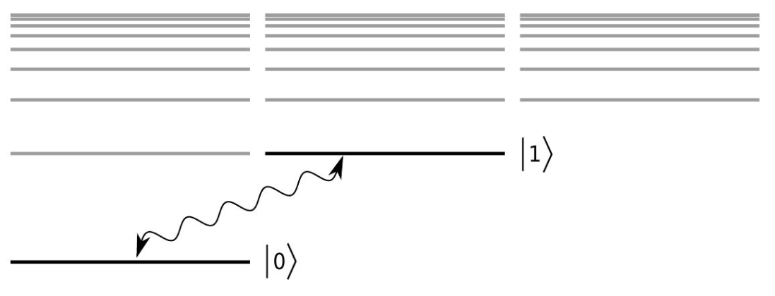
Figure \(\PageIndex{1}\): Energy level diagram of an atom. Ground state and first excited state correspond to qubit levels, \(|0\rangle\) and \(|1\rangle\), respectively.

Photon Polarization

Classically, a photon may be described as a traveling electromagnetic wave. This description can be fleshed out using Maxwell's equations, but for our purposes we will focus simply on the fact that an electromagnetic wave has a polarization which describes the orientation of the electric field oscillations (see Fig. \(\PageIndex{2}\)). So, for a given direction of photon motion, the photon's polarization axis might lie anywhere in a 2-d plane perpendicular to that motion. It is thus natural to pick an orthonormal 2-d basis (such as \(\vec{x}\) and \(\vec{y}\), or "vertical" and "horizontal") to describe the polarization state (i.e. polarization direction) of a photon. In a quantum mechanical description, this 2-d nature of the photon polarization is represented by a qubit, where the amplitude of the overall polarization state in each basis vector is just the projection of the polarization in that direction.

The polarization of a photon can be measured by using a polaroid film or a calcite crystal. A suitably oriented polaroid sheet transmits x-polarized photons and absorbs y-polarized photons. Thus a photon that is in a superposition \(|\phi\rangle=\alpha|\mathrm{x}\rangle+\beta|\mathrm{y}\rangle\) is transmitted with probability \(|\alpha|^{2}\). If the photon now encounters another polariod sheet with the same orientation, then it is transmitted with probability 1 . On the other hand, if the second polaroid sheet has its axes crossed at right angles to the first one, then if the photon is transmitted by the first polaroid, then it is definitely absorbed by the second sheet. This pair of polarized sheets at right angles thus blocks all the light. A somewhat counter-intuitive result is now obtained by interposing a third polariod sheet at a 45 degree angle between the first two. Now a photon that is transmitted by the first sheet makes it through the next two with probability
\(1 / 4\).

Figure \(\PageIndex{2}\): Using the polarization state of light as the qubit. Horizontal polarization corresponds to qubit state, \(|\hat{x}\rangle\), while vertical polarization corresponds to qubit state, \(|\hat{y}\rangle\).

To see this first observe that any photon transmitted through the first filter is in the state, \(|0\rangle\). The probability this photon is transmitted through the second filter is \(1 / 2\) since it is exactly the probability that a qubit in the state \(|0\rangle\) ends up in the state \(|+\rangle\) when measured in the \(|+\rangle,|-\rangle\) basis. We can repeat this reasoning for the third filter, except now we have a qubit in state \(|+\rangle\) being measured in the \(|0\rangle,|1\rangle\)-basis - the chance that the outcome is \(|0\rangle\) is once again \(1 / 2\).

Spins

Like photon polarization, the spin of a (spin-1/2) particle is a two-state system, and can be described by a qubit. Very roughly speaking, the spin is a quantum description of the magnetic moment of an electron which behaves like a spinning charge. The two allowed states can roughly be thought of as clockwise rotations ("spin-up") and counter clockwise rotations ("spin-down"). We will say much more about the spin of an elementary particle later in the course.

Measurement Example I: Phase Estimation

Now that we have discussed qubits in some detail, we can are prepared to look more closesly at the measurement principle. Consider the quantum state,

\[|\psi\rangle=\frac{1}{\sqrt{2}}|0\rangle+\frac{e^{i \theta}}{\sqrt{2}}|1\rangle\]

If we were to measure this qubit in the standard basis, the outcome would be 0 with probability \(1 / 2\) and 1 with probability \(1 / 2\). This measurement tells us only about the norms of the state amplitudes. Is there any measurement that yields information about the phase, \(\theta\) ?

To see if we can gather any phase information, let us consider a measurement in a basis other than the standard basis, namely

\[|+\rangle \equiv \frac{1}{\sqrt{2}}(|0\rangle+|1\rangle) \quad \text { and } \quad|-\rangle \equiv \frac{1}{\sqrt{2}}(|0\rangle-|1\rangle)\]

What does \(|\phi\rangle\) look like in this new basis? This can be expressed by first writing,

\[|0\rangle=\frac{1}{\sqrt{2}}(|+\rangle+|-\rangle) \quad \text { and } \quad|1\rangle=\frac{1}{\sqrt{2}}(|+\rangle-|-\rangle) \text {. }\]

Now we are equipped to rewrite \(|\psi\rangle\) in the \(\{|+\rangle,|-\rangle\}\)-basis,

\[
\begin{align}
|\psi\rangle & \left.=\frac{1}{\sqrt{2}}|0\rangle+\frac{e^{i \theta}}{\sqrt{2}}|1\rangle\right) \\ \notag \\
& =\frac{1}{2}(|+\rangle+|-\rangle)+\frac{e^{i \theta}}{2}(|+\rangle-|-\rangle) \\ \notag \\
& =\frac{1+e^{i \theta}}{2}|+\rangle+\frac{1-e^{i \theta}}{2}|-\rangle .
\end{align}
\]

Recalling the Euler relation, \(e^{i \theta}=\cos \theta+i \sin \theta\), we see that the probability of measuring \(|+\rangle\) is \(\frac{1}{4}\left((1+\cos \theta)^{2}+\sin ^{2} \theta\right)=\cos ^{2}(\theta / 2)\). A similar calculation reveals that the probability of measuring \(|-\rangle\) is \(\sin ^{2}(\theta / 2)\). Measuring in the \((|+\rangle,|-\rangle)\)-basis therefore reveals some information about the phase \(\theta\).

Later we shall show how to analyze the measurement of a qubit in a general basis.

Measurement example II: General Qubit Bases

What is the result of measuring a general qubit state \(|\psi\rangle=\alpha|0\rangle+\beta|1\rangle\), in a general orthonormal basis \(|v\rangle,\left|v^{\perp}\right\rangle\), where \(|v\rangle=a|0\rangle+b|1\rangle\) and \(\left|v^{\perp}\right\rangle=\) \(b^{*}|0\rangle-a^{*}|1\rangle\) ? You should also check that \(|v\rangle\) and \(\left|v^{\perp}\right\rangle\) are orthogonal by showing that \(\left\langle v^{\perp} \mid v\right\rangle=0\).

To answer this question, let us make use of our recently acquired braket notation. We first show that the states \(|v\rangle\) and \(\left|v^{\perp}\right\rangle\) are orthogonal, that is, that their inner product is zero:

\[
\begin{align}
\left\langle v^{\perp} \mid v\right\rangle & =\left(b^{*}|0\rangle-a^{*}|1\rangle\right)^{\dagger}(a|0\rangle+b|1\rangle) \\ \notag \\
& =\left(b \left\langle0|-a\langle 1|)^{\dagger}(a|0\rangle+b|1\rangle)\right.\right. \\ \notag \\
& =b a\langle 0 \mid 0\rangle-a^{2}\langle 1 \mid 0\rangle+b^{2}\langle 0 \mid 1\rangle-a b\langle 1 \mid 1\rangle \\ \notag \\
& =b a-0+0-a b \\ \notag \\
& =0
\end{align}
\]

Here we have used the fact that \(\langle i \mid j\rangle=\delta_{i j}\).

Now, the probability of measuring the state \(|\psi\rangle\) and getting \(|v\rangle\) as a result is,

\[
\begin{align}
P_{\psi}(v) & =|\langle v \mid \psi\rangle|^{2} \\ \notag \\
& =\left|\left(a ^ { * } \left\langle\left.0\left|+b^{*}\langle 1|\right)(\alpha|0\rangle+\beta|1\rangle)\right|^{2}\right.\right.\right. \\ \notag \\
& =\left|a^{*} \alpha+b^{*} \beta\right|^{2}
\end{align}
\]

Similarly,

\[
\begin{align}
P_{\psi}\left(v^{\perp}\right) & =\left|\left\langle v^{\perp} \mid \psi\right\rangle\right|^{2} \\ \notag \\
& =\left|\left(b \left\langle\left.0|-a\langle 1|)(\alpha|0\rangle+\beta|1\rangle)\right|^{2}\right.\right.\right. \\ \notag \\
& =|b \alpha-a \beta|^{2}
\end{align}
\]