
11.7: Gauss' Law In Differential Form
- Page ID
- 972

\( \newcommand{\vecs}[1]{\overset { \scriptstyle \rightharpoonup} {\mathbf{#1}} } \)
\( \newcommand{\vecd}[1]{\overset{-\!-\!\rightharpoonup}{\vphantom{a}\smash {#1}}} \)
\( \newcommand{\dsum}{\displaystyle\sum\limits} \)
\( \newcommand{\dint}{\displaystyle\int\limits} \)
\( \newcommand{\dlim}{\displaystyle\lim\limits} \)
\( \newcommand{\id}{\mathrm{id}}\) \( \newcommand{\Span}{\mathrm{span}}\)
( \newcommand{\kernel}{\mathrm{null}\,}\) \( \newcommand{\range}{\mathrm{range}\,}\)
\( \newcommand{\RealPart}{\mathrm{Re}}\) \( \newcommand{\ImaginaryPart}{\mathrm{Im}}\)
\( \newcommand{\Argument}{\mathrm{Arg}}\) \( \newcommand{\norm}[1]{\| #1 \|}\)
\( \newcommand{\inner}[2]{\langle #1, #2 \rangle}\)
\( \newcommand{\Span}{\mathrm{span}}\)
\( \newcommand{\id}{\mathrm{id}}\)
\( \newcommand{\Span}{\mathrm{span}}\)
\( \newcommand{\kernel}{\mathrm{null}\,}\)
\( \newcommand{\range}{\mathrm{range}\,}\)
\( \newcommand{\RealPart}{\mathrm{Re}}\)
\( \newcommand{\ImaginaryPart}{\mathrm{Im}}\)
\( \newcommand{\Argument}{\mathrm{Arg}}\)
\( \newcommand{\norm}[1]{\| #1 \|}\)
\( \newcommand{\inner}[2]{\langle #1, #2 \rangle}\)
\( \newcommand{\Span}{\mathrm{span}}\) \( \newcommand{\AA}{\unicode[.8,0]{x212B}}\)
\( \newcommand{\vectorA}[1]{\vec{#1}} % arrow\)
\( \newcommand{\vectorAt}[1]{\vec{\text{#1}}} % arrow\)
\( \newcommand{\vectorB}[1]{\overset { \scriptstyle \rightharpoonup} {\mathbf{#1}} } \)
\( \newcommand{\vectorC}[1]{\textbf{#1}} \)
\( \newcommand{\vectorD}[1]{\overrightarrow{#1}} \)
\( \newcommand{\vectorDt}[1]{\overrightarrow{\text{#1}}} \)
\( \newcommand{\vectE}[1]{\overset{-\!-\!\rightharpoonup}{\vphantom{a}\smash{\mathbf {#1}}}} \)
\( \newcommand{\vecs}[1]{\overset { \scriptstyle \rightharpoonup} {\mathbf{#1}} } \)
\(\newcommand{\longvect}{\overrightarrow}\)
\( \newcommand{\vecd}[1]{\overset{-\!-\!\rightharpoonup}{\vphantom{a}\smash {#1}}} \)
\(\newcommand{\avec}{\mathbf a}\) \(\newcommand{\bvec}{\mathbf b}\) \(\newcommand{\cvec}{\mathbf c}\) \(\newcommand{\dvec}{\mathbf d}\) \(\newcommand{\dtil}{\widetilde{\mathbf d}}\) \(\newcommand{\evec}{\mathbf e}\) \(\newcommand{\fvec}{\mathbf f}\) \(\newcommand{\nvec}{\mathbf n}\) \(\newcommand{\pvec}{\mathbf p}\) \(\newcommand{\qvec}{\mathbf q}\) \(\newcommand{\svec}{\mathbf s}\) \(\newcommand{\tvec}{\mathbf t}\) \(\newcommand{\uvec}{\mathbf u}\) \(\newcommand{\vvec}{\mathbf v}\) \(\newcommand{\wvec}{\mathbf w}\) \(\newcommand{\xvec}{\mathbf x}\) \(\newcommand{\yvec}{\mathbf y}\) \(\newcommand{\zvec}{\mathbf z}\) \(\newcommand{\rvec}{\mathbf r}\) \(\newcommand{\mvec}{\mathbf m}\) \(\newcommand{\zerovec}{\mathbf 0}\) \(\newcommand{\onevec}{\mathbf 1}\) \(\newcommand{\real}{\mathbb R}\) \(\newcommand{\twovec}[2]{\left[\begin{array}{r}#1 \\ #2 \end{array}\right]}\) \(\newcommand{\ctwovec}[2]{\left[\begin{array}{c}#1 \\ #2 \end{array}\right]}\) \(\newcommand{\threevec}[3]{\left[\begin{array}{r}#1 \\ #2 \\ #3 \end{array}\right]}\) \(\newcommand{\cthreevec}[3]{\left[\begin{array}{c}#1 \\ #2 \\ #3 \end{array}\right]}\) \(\newcommand{\fourvec}[4]{\left[\begin{array}{r}#1 \\ #2 \\ #3 \\ #4 \end{array}\right]}\) \(\newcommand{\cfourvec}[4]{\left[\begin{array}{c}#1 \\ #2 \\ #3 \\ #4 \end{array}\right]}\) \(\newcommand{\fivevec}[5]{\left[\begin{array}{r}#1 \\ #2 \\ #3 \\ #4 \\ #5 \\ \end{array}\right]}\) \(\newcommand{\cfivevec}[5]{\left[\begin{array}{c}#1 \\ #2 \\ #3 \\ #4 \\ #5 \\ \end{array}\right]}\) \(\newcommand{\mattwo}[4]{\left[\begin{array}{rr}#1 \amp #2 \\ #3 \amp #4 \\ \end{array}\right]}\) \(\newcommand{\laspan}[1]{\text{Span}\{#1\}}\) \(\newcommand{\bcal}{\cal B}\) \(\newcommand{\ccal}{\cal C}\) \(\newcommand{\scal}{\cal S}\) \(\newcommand{\wcal}{\cal W}\) \(\newcommand{\ecal}{\cal E}\) \(\newcommand{\coords}[2]{\left\{#1\right\}_{#2}}\) \(\newcommand{\gray}[1]{\color{gray}{#1}}\) \(\newcommand{\lgray}[1]{\color{lightgray}{#1}}\) \(\newcommand{\rank}{\operatorname{rank}}\) \(\newcommand{\row}{\text{Row}}\) \(\newcommand{\col}{\text{Col}}\) \(\renewcommand{\row}{\text{Row}}\) \(\newcommand{\nul}{\text{Nul}}\) \(\newcommand{\var}{\text{Var}}\) \(\newcommand{\corr}{\text{corr}}\) \(\newcommand{\len}[1]{\left|#1\right|}\) \(\newcommand{\bbar}{\overline{\bvec}}\) \(\newcommand{\bhat}{\widehat{\bvec}}\) \(\newcommand{\bperp}{\bvec^\perp}\) \(\newcommand{\xhat}{\widehat{\xvec}}\) \(\newcommand{\vhat}{\widehat{\vvec}}\) \(\newcommand{\uhat}{\widehat{\uvec}}\) \(\newcommand{\what}{\widehat{\wvec}}\) \(\newcommand{\Sighat}{\widehat{\Sigma}}\) \(\newcommand{\lt}{<}\) \(\newcommand{\gt}{>}\) \(\newcommand{\amp}{&}\) \(\definecolor{fillinmathshade}{gray}{0.9}\)Gauss' law is a bit spooky. It relates the field on the Gaussian surface to the charges inside the surface. What if the charges have been moving around, and the field at the surface right now is the one that was created by the charges in their previous locations? Gauss' law --- unlike Coulomb's law --- still works in cases like these, but it's far from obvious how the flux and the charges can still stay in agreement if the charges have been moving around.
For this reason, it would be more physically attractive to restate Gauss' law in a different form, so that it related the behavior of the field at one point to the charges that were actually present at that point. This is essentially what we were doing in the fable of the flea named Gauss: the fleas' plan for surveying their planet was essentially one of dividing up the surface of their planet (which they believed was flat) into a patchwork, and then constructing small a Gaussian pillbox around each small patch. The equation \(E_{\perp}=2\pi k\sigma\) then related a particular property of the local electric field to the local charge density.
In general, charge distributions need not be confined to a flat surface --- life is three-dimensional --- but the general approach of defining very small Gaussian surfaces is still a good one. Our strategy is to divide up space into tiny cubes, like the one on page 621. Each such cube constitutes a Gaussian surface, which may contain some charge. Again we approximate the field using its six values at the center of each of the six sides. Let the cube extend from \(x\) to \(x+dx\), from \(y\) to \(y+dy\), and from \(y\) to \(y+dy\).
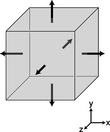
a / A tiny cubical Gaussian surface.
The sides at \(x\) and \(x+dx\) have area vectors \(-dydz\hat{\mathbf{x}}\) and \(dydz\hat{\mathbf{x}}\), respectively. The flux through the side at \(x\) is \(-E_x(x)dydz\), and the flux through the opposite side, at \(x+dx\) is \(E_x(x+dx)dydz\). The sum of these is \((E_x(x+dx)-E_x(x))dydz\), and if the field was uniform, the flux through these two opposite sides would be zero. It will only be zero if the field's \(x\) component changes as a function of \(x\). The difference \(E_x(x+dx)-E_x(x)\) can be rewritten as \(dE_x=(dE_x)/(dx)dx\), so the contribution to the flux from these two sides of the cube ends up being
\[\begin{equation*} \frac{dE_x}{dx}dxdydz . \end{equation*}\]
Doing the same for the other sides, we end up with a total flux
\[\begin{align*} d \Phi &= \left(\frac{dE_x}{dx}+\frac{dE_y}{dy} +\frac{dE_z}{dz}\right)dxdydz \\ &= \left(\frac{dE_x}{dx}+\frac{dE_y}{dy} +\frac{dE_z}{dz}\right)dv ,\end{align*}\]
where \(dv\) is the volume of the cube. In evaluating each of these three derivatives, we are going to treat the other two variables as constants, to emphasize this we use the partial derivative notation \(\partial\) introduced in chapter 3,
\[\begin{align*} d \Phi &= \left(\frac{\partial E_x}{\partial x}+\frac{\partial E_y}{\partial y} +\frac{\partial E_z}{\partial z}\right)dv .\\ \text{Using Gauss' law,} \\ 4\pi k q_{in} &= \left(\frac{\partial E_x}{\partial x}+\frac{\partial E_y}{\partial y} +\frac{\partial E_z}{\partial z}\right)dv ,\end{align*}\]
and we introduce the notation \(\rho\) (Greek letter rho) for the charge per unit volume, giving
\[\begin{align*} 4\pi k \rho &= \frac{\partial E_x}{\partial x}+\frac{\partial E_y}{\partial y} +\frac{\partial E_z}{\partial z} . \end{align*}\]
The quantity on the right is called the divergence of the electric field, written \(\rm div \mathbf{E}\). Using this notation, we have \(\rm div \mathbf{E} = 4\pi k \rho .\)
This equation has all the same physical implications as Gauss' law. After all, we proved Gauss' law by breaking down space into little cubes like this. We therefore refer to it as the differential form of Gauss' law, as opposed to \(\Phi=4\pi kq_{in}\), which is called the integral form.
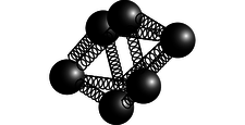
b / A meter for measuring \(\rm div \mathbf{E}\).
Figure b shows an intuitive way of visualizing the meaning of the divergence. The meter consists of some electrically charged balls connected by springs. If the divergence is positive, then the whole cluster will expand, and it will contract its volume if it is placed at a point where the field has \(\rm div \mathbf{E}\lt0\). What if the field is constant? We know based on the definition of the divergence that we should have \(\rm div \mathbf{E}=0\) in this case, and the meter does give the right result: all the balls will feel a force in the same direction, but they will neither expand nor contract.
| Example 36: Divergence of a sine wave |
|---|
|
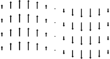
c / Example 36. \(\triangleright\) Figure c shows an electric field that varies as a sine wave. This is in fact what you'd see in a light wave: light is a wave pattern made of electric and magnetic fields. (The magnetic field would look similar, but would be in a plane perpendicular to the page.) What is the divergence of such a field, and what is the physical significance of the result? \(\triangleright\) Intuitively, we can see that no matter where we put the div-meter in this field, it will neither expand nor contract. For instance, if we put it at the center of the figure, it will start spinning, but that's it. Mathematically, let the \(x\) axis be to the right and let \(y\) be up. The field is of the form \[\begin{equation*} \mathbf{E} = (\text{sin} Kx)\: \hat{\mathbf{y}} , \end{equation*}\] where the constant \(K\) is not to be confused with Coulomb's constant. Since the field has only a \(y\) component, the only term in the divergence we need to evaluate is \[\begin{equation*} \mathbf{E} = \frac{\partial E_{y}}{\partial y} , \end{equation*}\] but this vanishes, because \(E_y\) depends only on \(x\), not \(y\) : we treat \(y\) as a constant when evaluating the partial derivative \(\partial E_{y}/\partial y\), and the derivative of an expression containing only constants must be zero. Physically this is a very important result: it tells us that a light wave can exist without any charges along the way to “keep it going.” In other words, light can travel through a vacuum, a region with no particles in it. If this wasn't true, we'd be dead, because the sun's light wouldn't be able to get to us through millions of kilometers of empty space! |
| Example 37: Electric field of a point charge |
|---|
|
The case of a point charge is tricky, because the field behaves badly right on top of the charge, blowing up and becoming discontinuous. At this point, we cannot use the component form of the divergence, since none of the derivatives are well defined. However, a little visualization using the original definition of the divergence will quickly convince us that div \(E\) is infinite here, and that makes sense, because the density of charge has to be infinite at a point where there is a zero-size point of charge (finite charge in zero volume). At all other points, we have \[\begin{equation*} \mathbf{E} = \frac{ kq}{ r^2}\hat{\mathbf{r}} , \end{equation*}\] where \(\hat{\mathbf{r}}=\mathbf{r}/ r=( x\hat{\mathbf{x}}+ y\hat{\mathbf{y}}+ z\hat{\mathbf{z}})/ r\) is the unit vector pointing radially away from the charge. The field can therefore be written as \[\begin{align*} \mathbf{E} &= \frac{ kq}{ r^3}\hat{\mathbf{r}} \\ &= \frac{ kq( x\hat{\mathbf{x}}+ y\hat{\mathbf{y}}+ z\hat{\mathbf{z}})}{\left( x^2+ y^2+ z^2\right)^\text{3/2}} . \\ \text{The three terms in the divergence are all similar, e.g.,}\\ \frac{\partial E_{x}}{\partial x} &= kq\frac{\partial}{\partial x}\left[\frac{ x}{\left( x^2+ y^2+ z^2\right)^\text{3/2}}\right] \\ &= kq\left[\frac{1}{\left( x^2+ y^2+ z^2\right)^\text{3/2}}-\frac{3}{2}\:\frac{2 x^2}{\left( x^2+ y^2+ z^2\right)^\text{5/2}}\right] \\ &= kq\left( r^{-3}-3 x^2 r^{-5}\right) . \end{align*}\] Straightforward algebra shows that adding in the other two terms results in zero, which makes sense, because there is no charge except at the origin. |
Gauss' law in differential form lends itself most easily to finding the charge density when we are give the field. What if we want to find the field given the charge density? As demonstrated in the following example, one technique that often works is to guess the general form of the field based on experience or physical intuition, and then try to use Gauss' law to find what specific version of that general form will be a solution.
| Example 38: The field inside a uniform sphere of charge |
|---|
|
\(\triangleright\) Find the field inside a uniform sphere of charge whose charge density is \(\rho\). (This is very much like finding the gravitational field at some depth below the surface of the earth.) \(\triangleright\) By symmetry we know that the field must be purely radial (in and out). We guess that the solution might be of the form \[\begin{equation*} \mathbf{E} = br^ p\hat{\mathbf{r}} , \end{equation*}\] where \(r\) is the distance from the center, and \(b\) and \(p\) are constants. A negative value of \(p\) would indicate a field that was strongest at the center, while a positive \(p\) would give zero field at the center and stronger fields farther out. Physically, we know by symmetry that the field is zero at the center, so we expect \(p\) to be positive. As in the example 37, we rewrite \(\hat{\mathbf{r}}\) as \(\mathbf{r}/ r\), and to simplify the writing we define \(n= p-1\), so \[\begin{equation*} \mathbf{E} = br^ n\mathbf{r} . \end{equation*}\] Gauss' law in differential form is \[\begin{equation*} \rm div \mathbf{E} = 4\pi k\rho , \end{equation*}\] so we want a field whose divergence is constant. For a field of the form we guessed, the divergence has terms in it like \[\begin{align*} \frac{\partial E_{x}}{\partial x} &= \frac{\partial}{\partial x}\left( br^{n} x\right) \\ &= b\left( nr^{ n-1}\frac{\partial r}{\partial x} x+r^ n\right) \\ \end{align*}\] The partial derivative \(\partial r/\partial x\) is easily calculated to be \(x/ r\), so \[\begin{equation*} \frac{\partial E_{x}}{\partial x} = b\left( nr^{ n-2} x^2+r^ n\right) \end{equation*}\] Adding in similar expressions for the other two terms in the divergence, and making use of \(x^2+ y^2+ z^2= r^2\), we have \[\begin{equation*} \rm div \mathbf{E} = b( n+3) r^ n . \end{equation*}\] This can indeed be constant, but only if \(n\) is 0 or \(-3\), i.e., \(p\) is 1 or \(-2\). The second solution gives a divergence which is constant and zero : this is the solution for the outside of the sphere! The first solution, which has the field directly proportional to \(r\), must be the one that applies to the inside of the sphere, which is what we care about right now. Equating the coefficient in front to the one in Gauss' law, the field is \[\begin{equation*} \mathbf{E} = \frac{4\pi k\rho}{3} r\:\hat{\mathbf{r}} . \end{equation*}\] The field is zero at the center, and gets stronger and stronger as we approach the surface. |
Benjamin Crowell (Fullerton College). Conceptual Physics is copyrighted with a CC-BY-SA license.