4.2: Measuring Motion - the Doppler Shift

Learning Objectives

• You will know that spectra can be represented as ribbon or line plots
• You will know that the motion of sources and observers change the observed wavelengths and frequencies of light

What Do You Think: Doppler Shift

Ever wonder how scientists are able to measure the masses of stars or galaxies? Or how they detect planets around other stars, or how it is possible to determine the distance to a galaxy across the Universe? It turns out that these measurements have something in common with everyday experiences like the apparent change in pitch of a car horn honking as it passes you. We will explore how these very different things are related in the following section.

Imagine you are sitting in a boat on the ocean. The boat will rise and fall periodically because waves in the water lift it as they pass. Now, further imagine that the boat is in a harbor that is sheltered such that only waves from a certain direction and with a constant wavelength (or frequency) are allowed to enter. In that case, the boat will rise and fall with the frequency of the waves. Now imagine that the boat begins to sail directly into the oncoming waves. Will the frequency at which the boat rises and falls remain the same, or will it change?

If you examine the situation, you can probably convince yourself that the frequency will change. Since the boat is moving toward the waves, successive waves do not have to travel quite as far to reach the boat as they would if the boat were stationary; the boat rushes to meet them as they travel toward it. Thus, they reach the boat a bit sooner than they would, and the boat is forced up and down more often than when it was stationary. That is, as perceived by a person on the moving boat, the waves have a higher frequency than when the boat is stationary. The faster the boat moves toward the waves, the higher the frequency will be when measured on the boat.

Now consider the case where the boat moves in the same direction as the waves (but still slower than they move through the water). Each successive wave must catch the receding boat, and so it takes a little bit longer for the waves to reach the boat than it would if the boat were stationary. This causes the boat to go up and down more slowly than it otherwise would. A person on the boat would therefore measure a lower frequency for the waves. Similar to the previous case, the faster the boat moves, the bigger the effect. The faster the boat moves, the slower the frequency of the waves the sailor perceives. Of course, in the case where the boat moves at precisely the same speed as the waves, the waves can never catch the boat. In that case, the boat does not go up and down at all, and the sailor measures zero frequency for the waves.

Next, you will find a set of activities, each depicting a person in a boat and waves, but in different configurations.

Boat Wave Demonstration

A. Source of waves is stationary, observer moves.

In this case, the source of waves is far to the right of the screen, so far in fact that the waves arrive parallel to each other. The observer (the person in the boat) is able to move around the water.

In the bottom right corner, the frequency of the waves is displayed. Two numbers are given. The first is the frequency emitted by the source. The second is the frequency of the waves as measured by the observer.

Move the boat around with your mouse.

Play Activity

1.

2.

3.

B. Student discussion about a moving source.

Play Activity

C. Stationary observer, moving source.

2.

3.

4.

These examples are meant to illustrate how the frequency of any periodic source is shifted if the source and observer are in motion relative to each other. We considered waves in water, but the arguments would be similar for any other periodic signal, such as sound waves (as in Figure 4.1) or light waves. This effect was first explained by the Austrian physicist Christian Doppler in 1842 and it has come to be called the Doppler shift .

Figure 4.1: Sound waves from a car that is not moving (top) and one that is traveling forward (bottom). The moving car’s sound waves are Doppler shifted so that the sound waves are shifted to lower frequencies (longer wavelengths) with respect to Observer A and shifted to higher frequencies (shorter wavelengths) with respect to Observe R B. Credit: NASA/SSU/Aurore Simonnet.

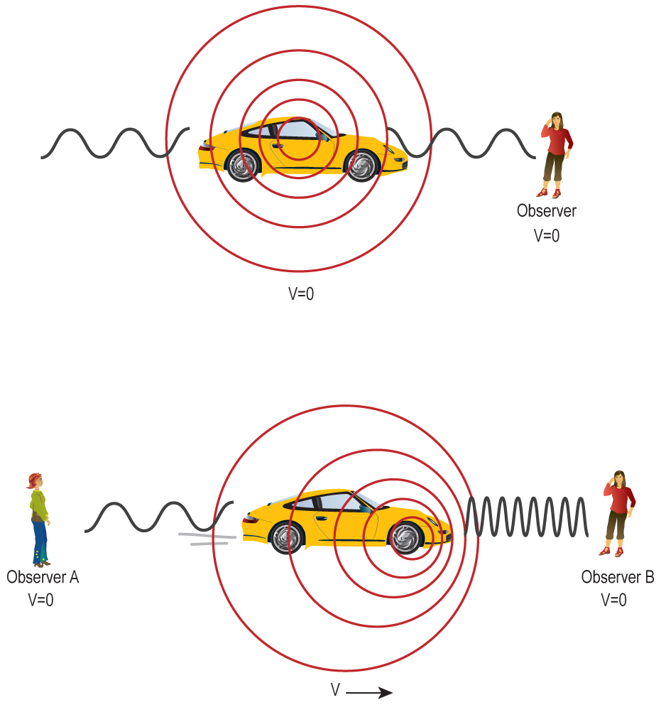
Doppler was working with sound, but the ideas also apply to light. Just as we considered successive water wave crests passing our boat, we can consider successive waves of light passing the boat. The same effect will be noted: The waves will pass by more frequently when we move toward the source, and they will arrive less frequently if we move away from the source.

A slight modification for light is that water waves and sound waves require a medium like air (or water) for the waves to travel upon. Light requires no such medium. As a result, the mathematical treatment of the Doppler shift in sound is slightly different from that for light, but the effect is qualitatively the same for both. Another difference is that light travels much faster than either water waves or sound, so the shift in the frequency of light is not generally large enough to notice without sensitive equipment.

When we observe light from a moving source, we can measure a shift in wavelength for specific absorption or emission lines and compare the observed wavelength to a reference wavelength, the one at which the lines would occur in the laboratory for an unmoving source. This reference wavelength is called the rest wavelength.

In the following equation, the Doppler shift (denoted by the letter \(z\)) is calculated by comparing (i.e., taking the ratio of) the difference (\(\Delta\lambda\)) between the observed wavelength (\(\lambda_{obs}\)) and the rest wavelength (\(\lambda\)).

\[z=\dfrac{Δλ}{λ}=\dfrac{λ_{obs}−λ}{λ}\nonumber \]

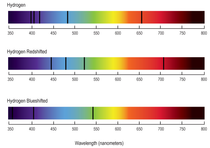
If the observed wavelength is greater than the rest wavelength, the Doppler shift will be a positive number. This indicates that the object is moving away from the observer. If the observed wavelength is longer than the rest wavelength, the shift is called “redshift.” On the other hand, if the object is moving toward the observer, \(z\) will be negative, and so will the velocity. In this case, we say that the spectrum is “blueshifted.” For historical reasons, the letter z is often called the “redshift” because in many astronomical examples, objects are moving away from Earth-bound observers. Also, “redshift” and “blueshift” do not mean exactly shifted to red and blue, they mean shifted to longer or shorter wavelengths, respectively. Figure 4.2 shows the spectrum of hydrogen at rest, redshifted, and blueshifted.

Figure 4.2: Three spectra. The spectrum of hydrogen in the visible portion of the electromagnetic spectrum. The top image shows the spectrum of hydrogen lines as seen in the lab (and therefore stationary). The second spectrum displays the hydrogen lines as seen from an object moving away from an observer. The third spectrum shows the hydrogen lines from an object moving toward an observer. Credit: NASA/SSU/Aurore Simonnet.

After we find the Doppler shift \(z\), we can calculate the velocity v of the moving object by multiplying the Doppler shift by the speed of light \(c\).

\[v=cz\nonumber \]

If the Doppler shift z is a positive number, then the velocity v will also be positive, meaning moving away. If v is negative, the object is moving toward the observer. We can also see from this equation that the bigger the velocity the greater the redshift and vice versa. This equation is valid as long as the speed is much less than c. For greater speeds, a more complicated variant of the equation must be used, but the two are the same at speeds much lower than the speed of light.

The Doppler shift has some important and useful consequences for the interpretation of the spectra emitted by celestial bodies. These will be explored in the next set of activities.

Doppler Shift of Hydrogen

Hydrogen atoms emit a series (“signature”) of spectral lines. When an object containing hydrogen is at rest relative to the observer, its spectrum has a red line (Line 1), a turquoise line (Line 2), a blue line (Line 3), and a series of purple lines. When an object is moving, this whole sequence is shifted in wavelength due to the Doppler effect.

In this activity, we will use the Spectrum Explorer tool to explore the motions of objects. Use the slider bar below the spectrum to Doppler shift the series of lines in order to check your predictions below.

Play Activity

1.

2.

3.

Often for quantitative work, it is more convenient to graph the intensity of light at each frequency or wavelength. Two ways of displaying the information in spectra are shown in Figure 4.3. In the next activity, you will practice converting between these two display methods.

Figure 4.3: Two ways to display information in spectra. Both depict the same colors, just displayed in different ways. The graph at the bottom numerically indicates the intensity of the light at each corresponding point on the “ribbon” spectrum at the top. For example, the dips in intensity on the bottom graph correspond to the dark bars on the top graph. Credit: NASA/SSU/Aurore Simonnet.

Two Ways of Representing a Spectrum

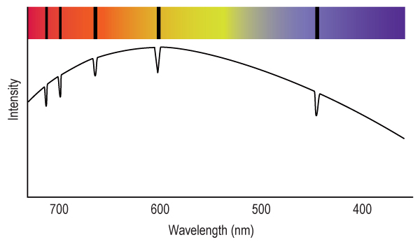
In modern times, astronomers rarely display spectra as a colorful ribbon of light with dark and bright bands. That was how spectra were displayed when they were gathered on photographic plates. With the advent of electronic detectors, which are easy to digitize, it became much easier to display spectra as a plot of intensity vs. wavelength.

This type of display has several advantages. First, it displays the intensity in an easily readable form (on the vertical axis). Inferring the intensity of a source across a ribbon spectrum is nearly impossible to do by eye. Second, very faint lines are more easily seen in line plots because they show up as slight dips or rises in intensity in some region. In ribbon plots, they can be extremely difficult to see. Finally, the strength of lines is more easily understood at a glance because the entire width of a line can be discerned on a graph, whereas this is difficult to do with the old ribbon plots.

To help you understand how ribbon plots correspond to line plots, we have created an interactive activity that allows you to convert a ribbon plot to a line plot. Use the activity as follows:

• Click the mouse on any point in the ribbon plot shown. The intensity of the light at that point will be plotted at the appropriate wavelength on the axes below the ribbon.
• Do this for many points along the ribbon, and see how the plot spectrum is built up. Be especially careful as you plot the regions around emission or absorption lines because the intensity changes very quickly with wavelength in those regions. Astronomers use computer programs to manage this conversion procedure for the spectra they collect at telescopes.
• When you have what you believe to be enough sampled points on the ribbon plot, click the “Connect Points” button. The points will be connected, allowing you to view your completed spectrum.
• Another plot can be displayed in addition to yours by clicking the button labeled “Full Data .” This plot is generated by sampling along the entire spectrum, not using the discrete (and somewhat arbitrary) sampling you used.

In this activity, the wavelength scale is in Angstroms (Å), a unit commonly used by astronomers (1 Å = 10^-10 m).

Play Activity

1.

2.

3.

4.

The spectrum we have used for this activity is that of an A-type star, between about 3,500 and 4,200 Å. Vega is one example of such a star. We will be displaying spectra in the line format for the remainder of the modules.

Quantitative Doppler Shift

Your goal in this activity is to determine the velocities of several galaxies based on their spectra using the Doppler shift. A small part of each galaxy’s spectrum is provided, showing the \({\rm H\beta}\) (hydrogen beta) spectral line, which has a rest wavelength of 4,860 Å (1 Å = 10^-10 m). The top graph is that of a reference galaxy that has not been shifted. The lower graph displays the observed spectrum for the selected galaxy.

A galaxy can be chosen by double-clicking on it. You should see that the Hβ line has been shifted to longer wavelengths for each of the galaxies. Double-click the galaxy image when you have finished analyzing it, to get back to the entire selection of galaxies.

Play Activity

For each galaxy:

• Find the observed wavelength , λ_obs, for the Hβ line by hovering over the highest point of the Hβ line and reading off the corresponding wavelength.
• Calculate the shift in wavelength, Δ λ = λ_obs - λ, in the Hβ line.
• Calculate the redshift , z = Δ λ / λ, for the Hβ line.
• Use this redshift to find the “velocity ” in km/s using: v = cz. The speed of light , c = 3 × 10⁵ km/s.

Worked Example for Galaxy A:

• The observed wavelength measured from the spectrum is λ_obs = 4,950 Å.
• The rest wavelength for Hβ is 4,860 Å, so the shift is Δλ = 4,950 Å - 4,860 Å = 90 Å.
• The redshift is then given by z = Δλ/λ = 90 Å / 4,860 Å = 0.0185
• From the redshift, we can calculate the velocity of the galaxy: v = (3.0e5 km/s)(0.0185) = 5546 km/s. Since the value is positive, we know this is a redshift and the galaxy is moving away from us.

1.

2.

3.