10.3: What is Curvature?

What Do You Think: Flatness and Curvature

Curvature in 2D Space

We have seen that light should follow a curved path when there is a gravitational acceleration. We have also seen that the rate time passes depends upon the strength of gravity. You should be getting the idea that gravity does some unexpected things to both space and time. These effects are somewhat reminiscent of the ways that space and time are distorted in special relativity. However, once the relative motions are chosen in special relativity, the distortions are the same everywhere, and they never change. The distortion of spacetime is more complicated in general relativity. We say that spacetime is flat and static in special relativity. In contrast, spacetime is curved and dynamic in general relativity.

What is meant by flat and curved? In this section you will explore the meaning of these words in some detail in order to help you better understand what Einstein’s view of gravity is really all about.

You are accustomed to “flat” and “curved” objects in the world. You might think of a soccer field as being flat, whereas a soccer ball is curved. While the terms "flat" and "curved" have a specific scientific and mathematical meaning, the everyday view of curvature is useful in helping to understand curvature of spacetime. In fact, the description of curvature in higher-dimensional spaces (even those in which one of the dimensions is time!) is based entirely upon our (mathematical) description of curvature in the normal space in which we live.

Think for a moment about a soccer field and a soccer ball. What do we mean when we say that one of them is flat and that the other is curved? There are many technical aspects involved in the answer to this question, but fundamentally, the best way to think about curvature is that it has to do with the way we measure the distance between two points in a space. So, for instance, on the soccer field we know that the distance between two points will be given by the Pythagorean theorem.

\[d^2=\Delta x^2+\Delta y^2 \nonumber \]

The letter \(d\) represents the straight-line distance between the points, and \(Δx\) and \(Δy\) are the \(x\) and \(y\) separations between them on a coordinate grid. (Figure \(\PageIndex{1}\)). We will illustrate what we mean here with some examples in the next activity.

Figure \(\PageIndex{1}\): Left panel: On the surface of a soccer field, the distances between two players can be computed using the Pythagorean theorem. However, on a curved surface like that of a soccer ball (right panel), the distance between two points does not follow the same relation. Although the soccer ball looks like it is made of flat hexagonal and pentagonal pieces, in reality, they each bulge out a bit due to the pressure inside the ball and its stuffing. Credit: NASA/SSU/Aurore Simonnet

DISTANCE ON A SOCCER FIELD

Imagine that two soccer players are on a field, as depicted in Figure \(\PageIndex{2}\). We can use a grid of points and the Pythagorean theorem to calculate the distance between them.

Figure \(\PageIndex{2}\): This soccer field has the origin at the lower left corner, and the coordinates indicate the positions of two players. Credit: NASA/SSU/Aurore Simonnet

Worked Example:

1. If we take the origin of our coordinate system to be at the lower left corner of the field, then the red player is at (x = 20 m, y = 10 m). The yellow player is at (x = 60 m, y = 40 m). What is the distance between them?

• Given: Red: x = 20 m, y = 10 m; Yellow x = 60 m, y = 40 m
• Find: the distance between the two soccer players: d
• Concept: d² = (∆x)² + (∆y)²
• Solution: First compute ∆x and ∆y:
• Since the red player is at x = 20 m and the yellow player at x = 60 m, we have: ∆x = 60 m - 20 m = 40 m.
• Similarly, ∆y = 40 m - 10 m = 30 m.
• Now, from the Pythagorean relation we get: d² = (∆x)² + (∆y)² = (40 m)² + (30 m)² = 1600 m² + 900 m² = 2500 m²
• Taking the square root of both sides: d = 50 m

Questions

In the worked example we saw that the distance between the two soccer players was 50 meters. We assumed that the origin of our coordinate system was at the lower left of the soccer field. Now, assume that the origin is at the upper left to answer the following questions.

1.

2.

 

3.

 

It should be clear from the activity that the choice of coordinates will have no effect on the outcome. We can shift the coordinate origin around to any point we wish. We could even use a rotated coordinate system, one whose axes did not line up with the edges of the soccer field: the distances between the players would still be the same. It would have to be! This will also be true in curved spaces. However, in a curved space we will not be able to use the familiar Pythagorean relation. In curved spaces, distances are not related that way.

The surface of a soccer ball is an example of one kind of curved space: it is a sphere. If we know the positions of two points on a sphere, can we still compute the distance between them? We can, but the procedure is more complicated than it is for a flat soccer field.

Consider a larger sphere than a soccer ball, for example, Earth. Now think about the distances between points on Earth’s surface, perhaps the distances between cities. We can lay out an x–y grid on Earth’s surface just as we did on the soccer field. We might put the origin at the intersection of the Greenwich Meridian and the equator. Then we could measure the position of every point on Earth’s surface using that grid.

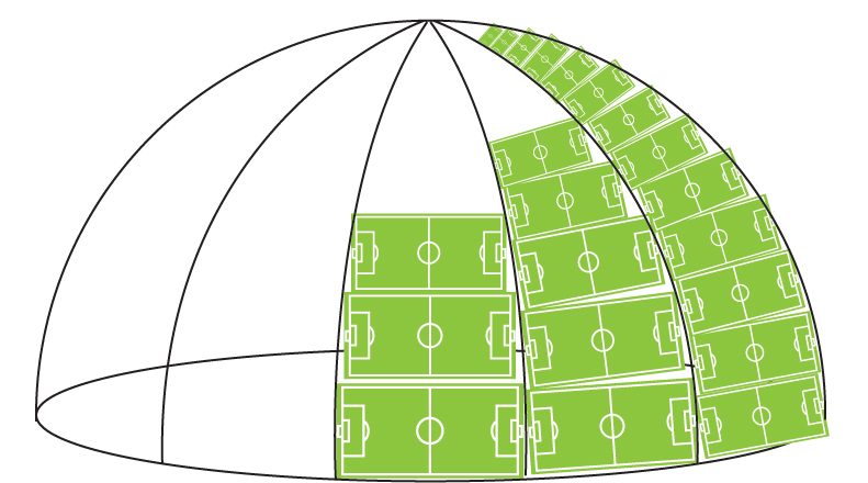
As a first try, you might lay out a lot of soccer fields, each touching the adjacent ones at its edges. You could build up a huge grid this way by matching the grid lines from one field to each adjacent field and simply attaching the coordinates of one field to the next. In this way, you could try to cover Earth with a grid of patchwork fields, like a big quilt. But would it work? Unfortunately, no. There is no way to cover Earth’s surface with flat, square soccer fields. If you try, you would find that some of the fields overlap, or else there are gaps between them. This is true no matter how small you make the fields. Even tiny ones will have some overlap or leave some gaps that they do not cover.

Figure \(\PageIndex{3}\): We cannot cover Earth’s surface with flat soccer fields. We have to deform the fields by stretching them in some places, compressing them in others. This is because soccer fields are flat, whereas Earth’s surface is curved. Credit: NASA/SSU/Aurore Simonnet

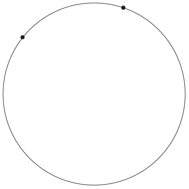
To understand why soccer fields cannot cover Earth’s surface, just think about the grid system that we actually do use on Earth’s surface: The grid is called longitude (perhaps like our x–coordinate on the soccer field) and latitude (like our y–coordinate). There is something a little peculiar about these coordinates, as we can see if we consider two pairs of points. The first pair has x = 10, y = 10 and x = 20, y = 10. The second pair of points has x = 10, y = 70, and x = 20, y = 70. Figure \(\PageIndex{4}\) shows how these points are laid out.

Figure \(\PageIndex{4}\): Two points separated by the same longitude near the equator (A and B) are farther from each other than two points with the same longitudes that are near the poles (C and D). Credit: NASA/SSU/Aurore Simonnet

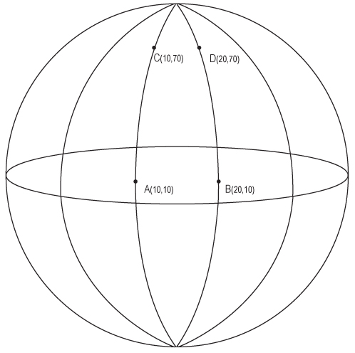
If this were flat space, then we know that the distance between the first two points would be the same as the distance between the second two. For both sets of points the y coordinate is the same, so the only difference lies in the x coordinate. In a flat space we would have d = ∆x = 10. But, that is not so on a sphere. The points near the pole are clearly closer together than the points near the equator. If you have a globe handy, have a look at it and you will see that this is true. And for an extreme example, if we had set the y value of the points to 90 degrees, then they would coincide; there would be no distance between them at all!

This property of coordinates in spherical geometries is distinctly different from the properties of coordinates in a flat coordinate system. In a flat system, lines that start out parallel remain so forever. In a spherical system, the lines of longitude that start out parallel at the equator do not remain so. In fact, they actually cross at the poles. The extreme example is two lines of longitude separated by 90 degrees: they start out parallel (i.e., they are both perpendicular to the same line, the equator), but when they reach the pole they are perpendicular and cross at a right angle.

If we insist on holding strictly onto ideas appropriate for flat spaces, the attributes of spherical ones seems a little bit absurd. Nonetheless, spherical geometries are real, and they do have these characteristics. They are simply different from the flat geometries with which most of us are more familiar. Probably the best thing we can do when learning about them is to relax our grip on some of the ideas instilled when we studied flat (Euclidean) geometry in school. And keep in mind that the geometry of general relativity, like that of a sphere, is definitely not Euclidean.

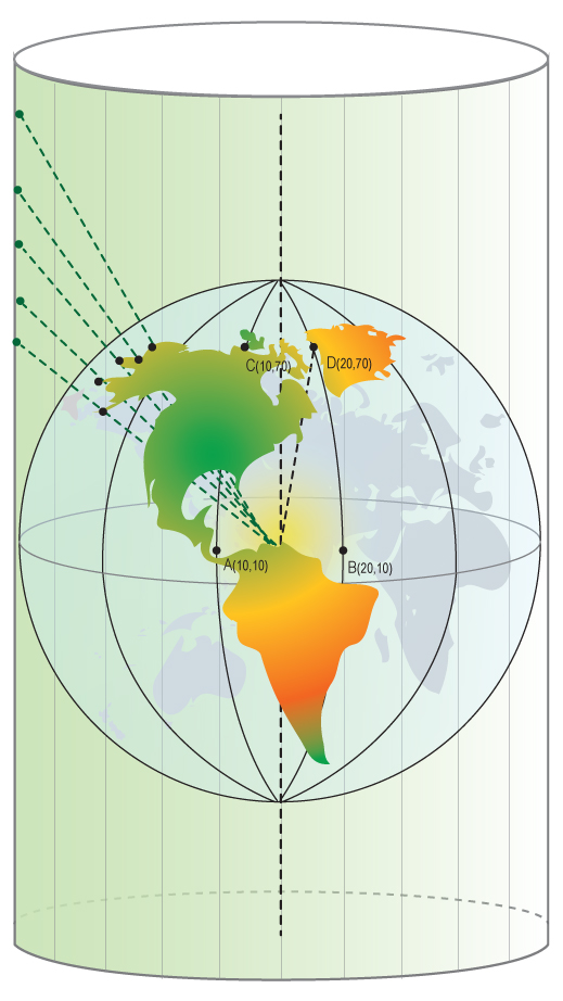
So how can we measure the distances between two points in a curved space? It must have something do to with the coordinates of the points. If it did not, there would not be any reason to use coordinates to describe the position of points. Have a look at the map of Earth’s surface in Figure \(\PageIndex{5}\). The map is a kind of projection that we often see on road maps or wall maps or books. To create this projection you can imagine a cylinder wrapped around Earth such that it just touches Earth’s surface at the equator, as in Figure \(\PageIndex{6}\). The points on the globe are projected out onto the cylinder to make the map. There are many ways to do this, and they have various advantages and disadvantages. However, none of them faithfully reproduces the distances between points over their entirety. There are always distortions introduced because the curved space of the sphere cannot be represented in the flat space of the cylinder without introducing warps or stretches. (Cylinders have flat geometry. We will explain this somewhat non-intuitive statement below.)

Figure \(\PageIndex{5}\): This kind of map is quite common. It projects the curved surface of Earth onto a flat map for ease of viewing. In doing so it distorts distances, with those near the pole appearing to be much larger than those near the equator. Credit: Shutterstock

In the projection we are using, called a Mercator projection, the distortions are noticeable because the parts of the map near the poles are represented as being much larger than they actually are relative to the parts near the equator. Put another way, distances near the poles appear to be much greater than they are on Earth’s surface. For instance, Greenland seems to be as big or bigger than South America. In fact it is roughly the size of Argentina.

To help the users of these maps take account of their distortions, map makers usually place a small scale somewhere on the map. The scale indicates how to read distances at various places on the map. So for example, the scale might indicate that near the equator one inch is equal to 100 kilometers, but at 70 degrees north of the equator this same one inch could correspond to 50 kilometers. Near the poles it takes more inches to represent a given distance, and objects look bigger because more inches are needed to represent them. It can be very misleading. This is an example of map coordinates not being related to map distances in a simple way, as they would be in a flat space. It is the essence of what we mean when we say a space is curved.

Figure \(\PageIndex{6}\): How a Mercator projection map is made, using a cylinder wrapped around a globe. Credit: NASA/SSU/Aurore Simonnet

For a sphere, writing down a scale for the coordinates is actually pretty simple, though the math needed to derive it is more than we want to tackle. We will just state that the correct way to find the distance \(d\) between two points on the surface of a sphere of radius \(R\), assuming small changes in latitude, \(\theta\), and longitude, \(\alpha\) is written as follows.

\[d^2=(R\Delta \theta)^2 + \cos^2\theta(R\Delta\alpha)^2 \nonumber \]

This expression does not differ so much from the Pythagorean relation we used in flat space. It still has the square of the distance related to the squares of the difference in coordinates, in this case \(\Delta\theta\) for the change in latitude and \(\Delta\alpha\) for the change in longitude. These must both be expressed in radians, not degrees, for the expression to be valid. (Remember that there are \(\pi\) radians in 180 degrees.) In addition, there is the radius of the sphere, \(R\). We need that to give us a size scale. After all, we travel farther going half way around Earth than we do going half way around a soccer ball, even though the change in coordinates amounts to 180 degrees in either case. But it is not the \(R\) that tells us the space is curved. The giveaway that we are dealing with a curved space is the \(\cos \theta\). It multiplies the longitude part of the distance, and it changes for different values of the latitude. But what does it do, exactly?

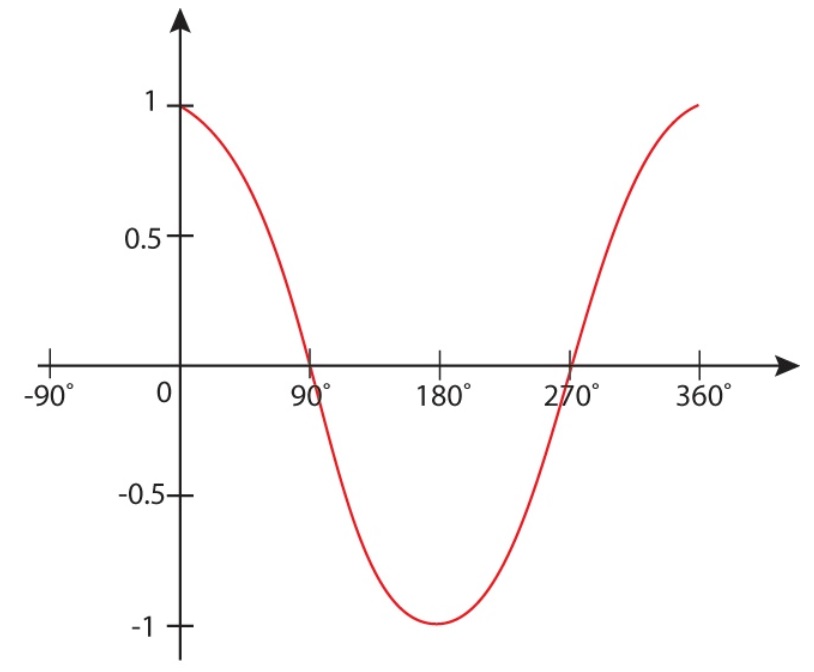
Remember that the cosine function varies between 1 and -1. It is 1 when its argument is zero (on the equator in this case) and it is zero when its argument is +90 degrees or -90 degrees, at the North or South Pole. Figure \(\PageIndex{7}\) shows a plot of the cosine for one complete trip around a circle, from zero to 360 degrees. If you go more than 360 degrees the cosine just repeats; it is just like you started counting again from zero every time you go once around the circle.

The cosine in the second term causes the longitude to make no contribution when for angles (latitudes) on either pole (where the cosine is zero), and it causes the change in longitude to have an equal effect with the change in latitude when the points are on the equator. In between the two the longitude contributes some, but not as much as the change in latitude.

So in effect, the cosine of the latitude scales the contribution of the change in longitude to the distance between two points. If you consider how longitude and latitude work on Earth’s surface, you will see that this is exactly what we expect. Lines of longitude get closer to each other as they leave the equator and approach the poles. Thus, we know that a difference in longitude will make a smaller contribution to the total distance between two points as the points approach the poles.

Figure \(\PageIndex{7}\): The cosine is a function of an angle. It varies between -1 and 1, and it repeats every 360 degrees. Credit: NASA/SSU/Aurore Simonnet

The following activity gives you a chance to use this relationship to find the distance between two points on the surface of a ball. Do not forget to convert the angles from degrees to radians (remember that \(\pi\) radians are 180 degrees).

Distance on a Soccer Ball

Worked Example:

1. Imagine there are two ants on the surface of a soccer ball. The ants are close to the “equator” of the soccer ball, at “latitude” +10 degrees. One ant is at “longitude” 10 degrees and the other is at 15 degrees, as measured in the soccer ball’s coordinate system. If the soccer ball is 22 cm in diameter, how far apart are the ants?

• Given:
  The radius of the soccer ball, R = 22 cm
  The ants are at coordinates (lat,long) = (10,10) and (10,15). These values are expressed in degrees, and we must convert them to radians so that we can use our distance relation:
  10 degrees = (10 degrees) (π radians / 180 degrees) = 0.1745 radians
  15 degrees = (15 degrees )(π radians / 180 degrees) = 0.2618 radians
• Find: The distance between the two coordinates, d
• Concept: We will use the expression for distance:
  d2=R2[(Δθ)2+cos2θ(Δα)2]
• Solution:
  First we need to find the cosine of the latitude, or cos(10) = 0.9848. Note that we do not have to convert the 10 degrees to radians when we take its cosine. The cosine of an angle is just a number. However, we must be careful to use the correct mode on our calculator when we take the cosine. Many scientific calculators can switch between using angles expressed in degrees or in radians. You can use either one, but make sure you know which your calculator is set to use.

Now we are ready to plug our numbers into the equation:

d² = R² (∆θ² + cos²θ ∆α²) = R² (0.1745 - 0.1745)² + (0.9848)² (0.2618 - 0.1745)² = 0.0075 R²

Taking the square root we get d = 0.0866 R. This is the separation of the two points in radians.

To find the distance between them in centimeters we have to multiply by the value for R, the radius of the ball:
d = (22 cm)(0.0866) = 1.9 cm

Questions

1.

2. W

 

If you wanted to be more precise, your simple cosine relation would not be good enough. In reality, the surface of Earth is not smooth; it is bumpy. It has mountains and valleys. Distances between points are affected by these, as you will have noticed if you ever had to hike over a mountain or down into a canyon to get to where you were going. It is not possible to write down a general relation for the distances between two points if we have to take into account these sorts of surface features. But that is okay, we know we could do it if we needed to, perhaps in some small area like that shown in Figure \(\PageIndex{8}\). We would just have to hire a surveyor to precisely map out the region of interest. Usually we do not have to know the geometry to that kind of precision, but in principle we could measure it.

Figure \(\PageIndex{8}\): If we wanted to measure the distance between two points on a bumpy surface we would have to know the curvature locally in that region. Generally we do not know this, although we could measure it if we wanted to. This figure of the Grand Canyon indicates a region where the Earth’s surface is bumpy. Credit: Shutterstock

Before we discuss curvature in spacetime, we want to illuminate one point that can cause confusion for people when they first learn these ideas about geometry. We said that we can project curved spaces like the surfaces of spheres onto cylinders to get a flat-space representation of them. But cylinders look curved, so how do we get a flat map by using a cylinder? The confusing part is that cylinders only look curved. In fact, cylinders are flat, at least geometrically speaking. From our definition of curvature— the way we measure distances in the space depends upon where we are— we can show that cylinders are flat.

The easiest way to understand how this works is to consider a flat piece of paper… We know that a piece of paper is flat because we can write down a coordinate system in which the distances between all the points are given by the familiar Pythagorean theorem. There are no extra terms anywhere— like the cosine term for spherical geometry, for instance. That is a flat space.

Now bend the piece of paper over so that opposite edges meet; we have made a cylinder. In doing this we did not have to distort the sheet of paper at all. We did not stretch it or crinkle it or tear it, we merely had to bend it so that the opposite sides coincided. This means that the distances between all the points are still related by the same Pythagorean relation, and the surface must still be flat. In general, a 2D space that can be “unfolded” or “unwrapped” and laid directly onto a flat space like a table without any distortions, like tearing, stretching or crinkling, must itself be a flat space.

Another important point relates to the use of the radius R as a scaling factor. A cylinder does have a radius, and a larger cylinder has a larger radius, as shown in Figure \(\PageIndex{9}\). We know that the bigger the cylinder, the larger the distance between any two points with coordinates (x,y). So the radius scales the distances to coincide with the size of the cylinder. However, the radius is constant over the entire surface we are considering. It is merely a constant multiplying, or scaling, factor that does not vary from point to point.

A sphere has a radius that scales distances too. This works the same way as it does for a cylinder: on a sphere the radius multiplies the longitude and the latitude parts of the distance relation and does not vary over the surface being scaled. However, on a sphere we also have the cosine term. It varies around the sphere and only multiplies the latitude term in the distance relation. Contrast that with the way the radius scales the size for both the cylinder and the sphere.

The critical difference between a curved space like the surface of a sphere and a flat space like the surface of a cylinder is that the former has extra terms that vary from place to place and that are required to compute distances between points in the space. This is what tells us that a sphere is curved, whereas a cylinder, lacking such terms, is flat.

Figure \(\PageIndex{9}\): (Left) If we wanted to measure the distance between two points on a cylindrical surface we would have to know the size of the cylinder in addition to the (x,y) coordinates of the individual points. (Right) Despite having a radius and looking curved, by our definition the cylinder has a flat geometry because it can be unrolled onto a flat surface Credit: NASA/SSU/Aurore Simonnet

We want to emphasize that when we talk about a space with a flat geometry, what we mean is that the distance between any two points is given by the Pythagorean theorem.

\[d^2=\Delta x^2+\Delta y^2 \nonumber \]

When we talk about a space with a curved geometry, we mean that the distance relation will have some other terms, A and B, where A and B in general would depend on the values of x and y.

\[d^2=A(x,y)\Delta x^2+B(x,y)\Delta y^2 \nonumber \]

In our example of the sphere, A was constant everywhere and equal to 1, and B was cos² θ. Here we are ignoring the scaling constant R because it just tells us about the size of the ball— Earth or soccer ball, say, just as in our description of the cylinder; it has nothing to do with the geometry or curvature.

Notice that we have not required our 2D space to exist in a 3D space in order to define the curvature. We can envision it that way if we like, and it seems a natural and convenient way to think about the surface of Earth. But it is not necessary.

What about the radius? Doesn't it imply some sort of curved surface? No, not necessarily. R has come in as a global scaling factor. We identify it as the radius of a ball, either Earth or a soccer ball in the examples above, but that is not essential. In general, R is just a number that tells us how large the distances in a space are. It is better to think of curvature in this way; once we go to curved spaces with more than two dimensions, it is not possible to visualize any higher dimensional spaces in which they might exist, so attempting to visualize them that way only leads to confusion.

Is a Circle Curved?

 

Figure \(\PageIndex{10}\): We generally think that the arc describing a circle is curved. Is this borne out using our more precise idea of what we mean by “curvature?” Credit: NASA/SSU/Aurore Simonnet

Distances and Curvature Extended to three Dimensions

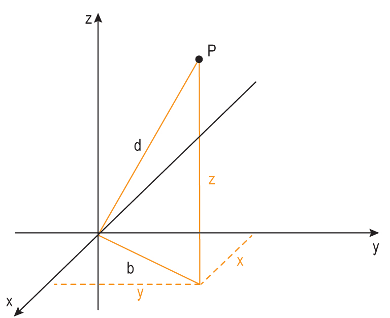
Everything we have said about 2-dimensional spaces can be generalized to three dimensions. The distance between two points in a flat 3-dimensional space is given by the 3D version of the Pythagorean theorem:

\[d^2=(Δx)^2+(Δy)^2+(Δz)^2 \nonumber \]

Figure \(\PageIndex{11}\): In three dimensions the Pythagorean theorem still applies. Notice how we can get a 3D version of the relation by successive applications in two-dimensional planes: b² + z² = d², and x² + y² = b², so x² + y² + z² = d². Credit: NASA/SSU/Aurore Simonnet

If the space is curved, then there could be extra multiplicative factors that depend on the coordinates, just as in 2 dimensions. We cannot easily draw an example of how that space might appear, but we could imagine and describe its behavior by adding appropriate extra terms to the distance relation. As an example:

\[d^2=A(x,y,z)(Δx)^2+B(x,y,z)(Δy)^2+C(x,y,z)(Δz)^2 \nonumber \]

In this relation A, B, and C depend on position (x,y,z), and they are different for different spaces; if A, B, and C are constant everywhere then the space is not curved. We can use expressions like this to compute distances between points in any space for which we know how A, B, and C vary with position. Vitally, we do not have to be able to actually visualize the space to do this.

We will worry about the detailed properties of curved 3-dimensional spaces. We mentioned it just as a bridge to describing the four curved dimensions of spacetime in general relativity. Curvature in 4-dimensional spaces can be described the same that it is in three dimensions.

Curvature in Spacetime

There are four spacetime dimensions: three of space, one of time. If we choose the x-direction to be in the direction of relative motion between different reference frames, then the other two dimensions are not affected by the motion, so we ignore them. Under this assumption, distances in spacetime are given by a relation reminiscent of the Pythagorean theorem, but with a negative sign on the time term.

\[s^2=(\Delta x)^2−(c\Delta t)^2 \nonumber \]

Here we label the distance in spacetime, or the spacetime interval, with the symbol s. The name helps us remember that it is different from a distance d in normal space, which has no time part.

For the case of special relativistic flat spacetime, it is easy to add in the other space dimensions if we wish. We do just what we did in the last section for normal 3D space:

\[s^2=(\Delta x)^2+(\Delta y)^2+(\Delta z)^2−(c\Delta t)2 \nonumber \]

The expression is a little bit more complicated than the previous one, and ignoring the y and z directions in special relativity allowed us to simplify our analysis somewhat without giving up a complete description of a system’s behavior. Unfortunately, we cannot do that in general relativity. Though it is always possible to take the relative velocity to define the x–direction in special relativity, the curvature of spacetime that is gravity is fundamentally bound up into the geometry of all four dimensions of spacetime. Just as the curvature on Earth’s surface depends on both latitude and longitude, we cannot describe it properly with just a single dimension. We must keep all four dimensions of spacetime to describe curvature in general relativity.

What are the extra terms that multiply the different parts of the expression to express the curvature in general relativity? That depends on the distribution of mass and energy, which are the sources of gravity. If we consider the gravity created by a spherical object like a star or planet. It will have a simple general form.

\[s^2=A[(\Delta x)^2+(\Delta y)^2+(\Delta z)^2]−B(c\Delta t)^2 \nonumber \]

In this case, we have already found the curvature term for the time part of the spacetime interval: In Section 10.2 we looked at how gravity curves time. That gave us an expression for the gravitational redshift, and that is exactly the distortion of the time dimension that we seek. Substituting in g = GM/r², we can write an expression for B.

\[B =\left(1-\frac{2GM}{rc^2}\right) \nonumber \]

We have expressed B using polar coordinates rather than Cartesian coordinates, for reasons that will be clear below. The spacetime interval, including the temporal curvature, can then be written as below.

\[s^2= A\left[\left(\Delta x\right)^2+\left(\Delta y\right)^2 + \left(\Delta z\right)^2\right] - \left(1-\frac{2GM}{rc^2}\right)\left(c\Delta t\right)^2 \nonumber \]

What about the spatial part of the interval? Does that also have to be modified? It turns out that it does, but there is no simple intuitive way to derive it. We would have to use the full mathematics of general relativity, and that is beyond the level of this unit. Instead we will simply state it, for later use, and note that the term seems reasonable given that it is the same as the temporal curvature term. Notice that for the spatial part we must divide rather than multiply by the curvature term.

\[s^2=\left(1-\frac{2GM}{rc^2}\right)^{-1}\left[\left(\Delta x\right)^2+\left(\Delta y\right)^2 + \left(\Delta z\right)^2\right]-\left(1-\frac{2GM}{rc^2}\right)\left(c\Delta t\right)^2 \nonumber \]

Using the fact that \(\left(\Delta r\right)^2 =\left(\Delta x\right)^2+\left(\Delta y\right)^2 + \left(\Delta z\right)^2\), we can express this interval in polar coordinates if we like.

\[s^2=\left(1-\frac{2GM}{rc^2}\right)^{-1}\left(\Delta r\right)^2-\left(1-\frac{2GM}{rc^2}\right)\left(c\Delta t\right)^2 \nonumber \]

This is the spacetime interval for a spherically symmetric object. The spherical symmetry means it is the same in all directions, x, y and z; they are all multiplied by the same curvature term, and that term depends only on the distance from the source, r, not on the direction. That is why polar coordinates are convenient. Also, note that the speed of light causes the curvature term to be very close to 1 in the Solar System. There is no object within the Solar System for which the ratio M/r is large enough to offset c², and it explains why we are generally not aware of curvature’s effects.

We will look at this interval and its consequences in much more detail in the next section on tests of general relativity.

The Gravitational Radius

If you take a look at the spacetime interval for a spherically symmetric object that we have just introduced, you notice that the curvature terms behave strangely at a certain point, namely, where r = 2GM/c². We call GM/c² the gravitational radius.

Notice that the gravitational radius depends on the mass of the object creating the gravity. The mass is a type of scaling factor; it plays a role similar to that the radius, R, did when measuring distances on the surface of a sphere or cylinder in the previous section.

Now let’s calculate the gravitational radius for some actual objects.

1. F

2.

3.