10.4: Tests of General Relativity

What Do You Think: Global Positioning System

In this section we will discuss some of the observational tests of the General Theory of Relativity. The theory makes a number of predictions about the world that are distinct from those of Newtonian gravity. We have already looked at several. Here we will consider a few more, and in somewhat greater detail. A number of these topics will be covered in later chapters, and this section serves as an introduction for deeper investigations to come.

The Orbit of Mercury

In 1915 when Einstein was completing his General Theory of Relativity, the orbit of Mercury had long been a puzzle to astronomers. Unlike the other planets, Mercury displays a slight variation in its orbit from the predictions of Newtonian gravitational theory. The orbit is not a closed ellipse as Newtonian theory predicts. It has a small amount of overshoot. This means that the entire orbit is slowly turning as the planet orbits the Sun. What we mean by this is that the point of closest approach to the Sun, called the perihelion, slowly rotates around the Sun, as does the point of greatest distance from the Sun, the aphelion (Figure \(\PageIndex{1}\)).

Figure \(\PageIndex{1}\): As Mercury orbits the Sun, its orbit slowly precesses around the Sun. This means that the position of the perihelion or aphelion slowly circles the Sun. Newtonian gravity cannot account for all of this motion, but general relativity does. The eccentricity of the orbit has been greatly exaggerated in this figure. Credit: NASA/SSU/Aurore Simonnet

The amount of this orbital shift is very small, and most of it is caused by gravitational tugs exerted by the other planets (primarily Jupiter), on Mercury as it goes around the Sun. However, even when the gravitational effects of the other planets are accounted for, Mercury still travels an extra 0.1036 arcseconds of rotation (beyond 360 degrees) for each orbit. This is an extremely small amount, too small to be seen, but it accumulates over time. After a century, Mercury will have rotated an extra 43 arcseconds beyond the predictions of Newtonian gravity. Even this angle is small, but it is measurable. The discrepancy indicates that something is not quite right with the Newtonian understanding of the Solar System.

The first attempts to account for Mercury’s orbital anomaly proposed the existence of a planet orbiting nearer to the Sun than Mercury. The planet, tentatively named Vulcan, was never seen, though many astronomers searched for it for many years. The idea of an unseen planet affecting the motion of a visible one was not unprecedented. The planet Neptune had been discovered in exactly this way. Astronomers had noticed anomalies in the position of Uranus. They were able to predict where an additional planet would have to be in order to cause those anomalies, and in 1846 Neptune was discovered in the area that had been predicted. A similar solution for Mercury’s strange motions was a reasonable suggestion, but no planet was ever found. The orbital anomalies remained an unsolved puzzle.

Albert Einstein was aware of Mercury’s anomalous orbit. When his new theory seemed complete enough to be applied to the orbit he did the calculation. There were no free parameters in Einstein’s theory that could be used to adjust it to the correct value. The only relevant inputs were the mass of the Sun and the size and eccentricity of Mercury’s orbit. When Einstein made the calculation, his theory predicted that Mercury should precess around the Sun at a rate of 43 arcseconds per century, precisely the amount of the observed anomaly.

This was one of the great moments in scientific discovery. Einstein’s theory, built from his imagination and tempered by his understanding of physics, could have been right or it could have been wrong. Only comparison with observations of nature would determine which. When Einstein made his calculation and his theory gave the correct answer, he knew that he had gained a profound insight into the workings of the world— he knew his theory was right. This was the culmination of 10 years of hard work, and on that evening in 1915, Einstein was the only person in the history of the world to have that insight. He would not remain so for long.

Light Bends Around the Sun

We have already discussed how, according to general relativity, gravity should cause light to follow a curved path. (See the discussion about the equivalence principle in Section 10.2.1.) However, we also showed that the expected deflection of a photon’s path on Earth is so small that it is completely unmeasurable. Earth simply does not produce enough spacetime curvature. Its mass is too small. If we could find an object with a larger mass, perhaps we could measure the deflection of a beam of light.

Fortunately, we have such an object quite close to us. The Sun is 300,000 times Earth’s mass, and there are many stars behind it that conveniently emit photons in all directions, including ours. Photons from these stars provide an excellent test of general relativity’s light-bending prediction. But is the Sun, massive as it is, able to create gravity strong enough to deflect starlight by a detectable amount?

We can make an estimate of the amount by which a beam of light will be deflected by the Sun. To do this, we will use the equivalence principle, as we did when we found the gravitational redshift in Section 10.2.2. We imagine that a beam of light begins its journey far away from the Sun, and that it passes close to the Sun as it travels. When it is close enough, it will begin to be affected by the Sun’s gravity. The beam will be deflected by some amount, just as we computed for a beam of light on Earth’s surface. The situation is shown schematically in Figure 10.18.

Figure \(\PageIndex{2}\): As a beam of light passes by a massive object like the Sun, it will be deflected from its original direction by an amount that depends on the mass of the gravitating object and the distance of closest approach. The trajectory of an undeflected photon is shown as the dotted path. Credit: NASA/SSU/Aurore Simonnet

If the photon were not deflected, then it would travel along the straight line indicated by the dotted path in Figure 10.18. However, the spacetime curvature bends that straight line into the curved path shown by the solid line. From the point of view of Newtonian gravity, we would say that the photon falls in the gravitational acceleration for some amount of time, and that its falling is what causes its direction to change.

Using the weak equivalence principle, we derive the angle of deflection in Going Further 10.3: Angle of Light Deflection. The total amount of deflection the photon experiences is given below.

\[\theta = \dfrac{2GM}{bc^2} \nonumber \]

The angle of deflection is represented by \(θ\), \(M\) is the mass of the Sun and \(b\) is the distance of closest approach. In the next activity, you will calculate the angle of deflection for the case of light passing close by the Sun.

Calculating Newtonian Deflection of Light

Newtonian arguments indicate that the angle \(\theta\) by which the light path should change as it travels near a massive body is given by \(\theta= 2GM/bc^2\), where M is the mass of the Sun (2 × 10³⁰ kg), and b is the distance of closest approach. Remember that \(\theta\) is given in radians.

Worked Example:

1. Calculate the angle θ (in radians) when b = the distance from the Sun to Earth = 1.5 × 10⁸ km.

• Given: b = 1.5E8 km = 1.5E11 m, M = 2E30, c = 3E8 m/s, G = 6.67E-11 Nm²/kg²
• Find: θ
• Concept: θ = 2GM/bc²
• Solution: θ = 2(6.67E-11 Nm²/kg²)(2E30 kg)/[(1.5E11 m)(3E8 m/s)²] = 1.98E-8 radians

Questions

1.

2.

The relationship used in this activity relies only the equivalence principle and our understanding of Newtonian gravity. It is remarkably close to the correct answer. In fact, what we have found is the amount by which Newtonian gravity alone would deflect light traveling close to the Sun. In doing so we have employed the curved-time part of the spacetime interval Recall that we were able to deduce time curvature using only the equivalence principle in Section 10.2.2.

However, in general relativity there is another curvature term that must be taken into account, that of space. The contribution of space curvature is the same size as the time curvature contribution, so it increases the deflection by a factor of two. The angle of deflection is very small, but it is large enough to be easily measurable, even with small telescopes.

The trouble, of course, is that we cannot usually view stars near the Sun. They are (obviously) up during the daytime, when the sky is bright enough to make the stars invisible. The situation changes during a total solar eclipse. For the brief few minutes that the Moon covers the Sun, it is possible to see stars near the solar limb.

In order to take advantage of rare solar eclipses, scientific expeditions were undertaken in 1919 to test this “light-bending” prediction of general relativity. Expeditions, under the direction of the British astronomer Arthur Eddington, traveled to the island of Principe, off the West Coast of Africa, and to Sobral, in Brazil, to view the eclipse. They photographed the sky around the Sun while the Moon covered it, and then compared the images to others taken at night, when the Sun was in another part of the sky. The results, though of poor quality, confirmed the predictions of general relativity. It was for this result that Albert Einstein became a household name and an icon. News of the eclipse results made huge headlines in newspapers around the world. Since the first measurements in 1919, the results have been confirmed several times with ever-improving precision. Modern measurements are generally done using radio telescopes and background galaxies.

The Sun is not the only object in the sky that deflects light as it travels to us. In fact, so-called gravitational lenses have become an important tool used by astronomers to study the Universe.

GOING FURTHER 10.4: NEWTONIAN GRAVITY AND CURVATURE

Gravitational Redshift

We have seen how the equivalence principle leads to a prediction of gravitational redshift — the shifting of light to lower frequency as it climbs out of a region of relatively stronger gravity to a region where gravity is weaker. The effect is too weak to be measured on Earth’s surface, as we calculated in Section 10.2.2. Even on the surface of the Sun, where gravity is more than 10 times greater than on Earth’s surface, the effect is too small to detect. However, nature has again provided us with a region where we can put the predictions of general relativity to the test.

When a star like the Sun dies, it leaves behind an object composed of the ash remaining from its lifetime of nuclear fusion. Such an object is called a white dwarf. The typical white dwarf is comparable in size to Earth, but has a mass comparable to the Sun's.

Surface Gravity of a White Dwarf

You should have found that the surface gravity of a white dwarf star is much larger than the gravity on Earth’s surface. If you recall, we deduced the gravitational redshift relation in Section 10.2.2 under the assumption that the gravity is weak. We also assumed that it was nearly constant. Neither of these assumptions is valid when we view the spectrum emitted at the surface of a white dwarf. Under these conditions we have to use the full expression for the gravitational redshift, valid for strong gravity as well as weak. That relationship is written below.

\[\lambda=\frac{\lambda_0}{\sqrt{1-\frac{2GM}{Rc^2}}} \nonumber \]

The measured wavelength, \(λ\), of a line is measured by an observer far away from the white dwarf, \(λ_0\) is the unshifted wavelength, \(R\) is the radius of the white dwarf, and \(M\) is its mass. \(G\) and \(c\) are the gravitational constant and speed of light, respectively. In the next activity we will employ this relationship to find the expected shift in the wavelength of a line in the white dwarf spectrum.

Gravitational Redshift on a White Dwarf

We can use the general relation for gravitational redshift, along with the value of the surface gravity of a white dwarf that you just found, to calculate the shift in wavelength of the sodium-D lines in the white dwarf spectrum. The sodium-D lines are two closely spaced lines that have rest wavelengths near 589 nm.

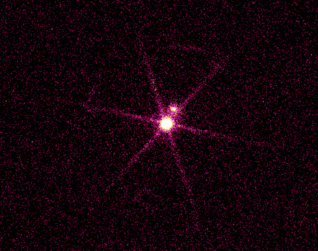
The measurement of the gravitational redshift of a white dwarf was first attempted in the 1920s for the companion of the star Sirius. At first the results seemed to agree with the predictions of general relativity. Later it was realized that the result was spurious, one reason being that most of the light being measured was from Sirius itself, not its faint companion star (see Figure \(\PageIndex{1}\)). In addition, the white dwarf radius used to compute the expected shift turned out to be wrong. More modern measurements using more powerful telescopes and detectors, as well as a better value for the radius of the white dwarf, have confirmed the predictions of general relativity. Ironically, the best constraints on the gravitational redshift turn out to have been done on Earth’s surface after all. These measurements used extremely sensitive equipment in a laboratory; the Pound-Rebka experiment was performed at Harvard University in 1959.

Figure \(\PageIndex{1}\): The figure on the left shows the Hubble Space Telescope image of Sirius A, the brightest star in our nighttime sky, along with its faint, tiny stellar companion, Sirius B. Astronomers overexposed the image of Sirius A [at center] so that the dim Sirius B [tiny dot at lower left] could be seen. The cross-shaped diffraction spikes and concentric rings around Sirius A, and the small ring around Sirius B, are artifacts produced within the telescope’s imaging system. Credit: NASA, H.E. Bond and E. Nelan (Space Telescope Science Institute, Baltimore, Md.); M. Barstow and M. Burleigh (University of Leicester, U.K.); and J.B. Holberg (University of Arizona) The figure on the right shows the Chandra X-ray Observatory image of the same two stars. In this case, however, the brighter star is Sirius B, which has a surface temperature of about 25,000 K, producing very low energy X-rays. The spike-like pattern is due to the support structure for Chandra’s transmission grating. Credit: NASA/SAO/CXC

Dragging of Reference Frames by Moving Objects

General relativity makes many predictions that seem strange to us. One of the strangest is called frame-dragging. Frame-dragging is also called the Lense-Thirring effect, after the two Austrian scientists, Josef Lense and Hans Thirring, who first studied it in 1918. Frame-dragging is the tendency of massive objects to pull space along with them as they move, sort of the way a boat pulls water along with it as it moves through the sea. It is clearly a tiny effect, since we are not aware of it at all from our normal experiences.

As a result of frame-dragging, spinning objects tend to wrap spacetime around them as they spin. Again, the effect tends to be so small as to be negligible in most cases. However, for a large object spinning rapidly, it is possible to measure the effects of frame-dragging with a sensitive enough experiment. Such an experiment, called Gravity Probe B (GPB), was conducted in Earth orbit during 2004 and 2005. GPB used sensitive gyroscopes to measure the effects of frame-dragging and confirmed the predictions of general relativity to its experimental precision, about 20%. For details about the GPB experiment, see Going Further 10.5: Gravity Probe B.

Note

The ideal gas law is easy to remember and apply in solving problems, as long as you get the proper values a

GOING FURTHER 10.5: GRAVITY PROBE B

Going Further 10.5: Gravity Probe B

The Gravity Probe B experiment was able to measure the extremely small frame-dragging effects from the spinning Earth. However, frame-dragging is not always a small effect. If an object is massive enough, and if it spins rapidly enough, then the effects of frame-dragging can be extreme. In these cases it can even be impossible to “sit still” in space because space itself is not sitting still: an observer would be forced along with the rapidly spinning space. Environments like that only exist close to rapidly spinning black holes, and we will consider those objects in the next chapter.

Gravitational Radiation

The final prediction of general relativity was only recently confirmed, in 2015, by direct measurement. To understand this prediction it is best to think first about Newton’s idea of gravity, described by his universal law of gravitation:

\[F_g=\frac{GM_1M_2}{r^2} \nonumber \]

There is nothing in this law that describes how the effects of gravity are transmitted from one place to another. In fact, according to this law, if we move one of the masses to a different point in space, then the other mass “knows” this instantly, and it reacts accordingly. The ability of gravity to act instantly - according to this law - across any distance bothered many of Newton's contemporaries. It continued to bother scientists who came after. And any scientists who lived after 1905, the year that Albert Einstein published his first paper on special relativity, knew that Newton’s law could not be correct. According to special relativity, it is not possible for any signal or information to cross space faster than light can travel.

In general relativity, gravity is not a force as envisioned by Newton. Instead, gravity is the result of spacetime being distorted, and the distortions of spacetime are caused by the distribution of mass. Changing the mass distribution will generally change the spacetime curvature, and thus also the gravitational effects on objects in that spacetime. However, when a mass distribution is changed, the effects of that change are not carried instantaneously to all points in space. The information is carried at the speed of light by ripples in the spacetime fabric. These ripples are called gravitational waves.

An analogy might help to understand how this works. We can imagine an observer living in a houseboat at the edge of the sea. If there is a storm far out to sea, the observer might not be aware of that fact. The storm could be over the horizon and out of view. However, storms generally have strong winds that create large waves. These waves travel outward from the storm in all directions, moving at speeds of a few meters per second. Eventually the waves will reach the shore where the observer lives, and the large swells will cause the houseboat to rock back and forth. In this way the observer might become aware of the storm’s existence even if the storm never approaches the shore at all— surfers are aware of this and use satellites to track storms so that they can predict when the waves at a certain beach might be good for surfing.

Replace the storm in our analogy with a binary star system and the surface of the sea with spacetime. You can see how we might be able to detect the stars, at least in principle, by measuring the rippling waves of spacetime caused by the stars’ motion. As the ripples pass us, the compressing and stretching of spacetime allows us to infer the existence of the stars even if we cannot see them by other means.

In practice, it is extremely difficult to detect the presence of gravitational waves. The stretching of spacetime is minuscule, and it tends to be swamped by non-gravitational effects. Most of these effects are local and have nothing to do with distant orbiting stars.

There are currently several experiments underway that are designed to measure gravitational waves directly. The first of these to have success is the Laser Interferometer Gravitational-wave Observatory, or LIGO. It detected a gravitational wave signal from a merging black hole system on September 14, 2015. To learn more about the LIGO experiment, see Going Further 10.6: Gravitational Wave Observatories.

Note

The ideal gas law is easy to remember and apply in solving problems, as long as you get the proper values a

GOING FURTHER 10.6: GRAVITATIONAL WAVE OBSERVATORIES

LIGO is the first experiment to detect gravitational waves directly, but even before this detection, scientists were sure the waves were there. The use of indirect means demonstrated the existence of the waves over the past several decades. This was somewhat analogous to the way a biologist might infer the presence of a bobcat if she saw its tracks or scat on a trail. Of course, gravitational waves don’t leave paw prints or other traces of their passing, but they do leave traces of themselves on the systems that emit them.

Let us return for a moment to the example of a binary star system. We said earlier that such a system would emit gravitational waves as the stars move in their orbits. These waves will carry energy. Since the waves are being produced by the movement of stars in space, the stars must be giving some of their own energy to the waves. There is no place else for the energy of the waves to come from.

If the stars lose energy to gravitational waves, then their motion will be affected. Different orbits have different amounts of energy, and the lower the energy of the orbit the smaller it is. So if binary stars create gravitational waves, then they must slowly spiral in toward each other as the waves carry the system’s energy away. Their orbital decay should be observable if we wait long enough.

In general, the in-spiraling of binary stars is difficult to measure. For instance, in the Solar System, the amount of energy loss from gravitational radiation is so small as to be utterly unimportant over the lifetime of the Sun, a period around 10 billion years. However, in some astrophysical systems the energy loss is quite a bit larger.

It turns out that the amount of energy radiated in gravitational waves is proportional to the square of the orbital frequency, or put another way, it depends on the size of the system. Larger systems have lower orbital frequencies, and so they produce fewer gravitational waves. This is one reason that the Solar System loses so little energy this way: the periods of the planets in the Solar System are months or years, making for tiny orbital frequencies. For certain systems though, the orbital frequency can be quite high.

Gravitational Luminosity

In this activity, we will calculate the amount of energy that could potentially be carried by gravitational radiation. We will compare our value with more familiar sources of radiation.

The energy emitted every second in gravitational waves by an object of mass m orbiting another of mass \(M\) is predicted by general relativity to be given by the expression below.

\[P_{gw}=\dfrac{2}{5}\left(\dfrac{GM}{Rc^2}\right)^5\left(\dfrac{m}{M}\right)^2\left(\frac{c^5}{G}\right) \nonumber \]

If we are considering a planet orbiting the Sun, then \(M\) is the mass of the Sun, \(m\) is the mass of the planet, and \(R\) is the size of the planet’s orbit. As usual, c and G are the speed of light and the gravitational constant, respectively. This expression is somewhat simplified if we rewrite it in terms of the gravitational radius.

\[P_{gw}=\frac{2}{5}\left(\frac{R_g}{R}\right)^5\left(\dfrac{m}{M}\right)^2\left(\frac{c^5}{G}\right) \nonumber \]

1.

2.

The previous activity demonstrated that gravitational radiation can in principle carry large amounts of energy. However, this is only important for certain kinds of systems. Such a system was discovered in the early 1970s by two scientists working at the Arecibo radio telescope in Puerto Rico, then the most sensitive radio telescope in the world. Sadly, that telescope collapsed in December of 2020 after suffering damage during Hurricane Maria in 2017.

The telescope was being employed in the 70s by a graduate student named Russell Hulse, who wished to find pulsars. These are rapidly rotating, highly magnetic neutron stars, the first examples of which had been discovered only a few years before by another graduate student in England, Jocelyn Bell. Pulars show flashes of emission analogous to those from a light house. They generally have very stable pulse separations that vary from a few seconds to tiny fractions of a second, depending on the object being observed. In fact, pulsar periods are so stable that they constitute the most accurate “clocks” known.

However, one of the pulsars discovered by Hulse, called PSR 1913+16, showed an unusual periodic variation in its pulse separation. Pulses would arrive slightly early on successive pulses, then switch and arrive slightly late. The early-late variation pattern repeated roughly every eight hours.

Upon discussing this pulsar with his advisor, Joseph Taylor, it became clear that what they were observing was a pulsar in orbit around another star. However, given the orbital period of only eight hours, the companion had to be extremely small. It was also dim, since no companion was visible. Further careful observations suggested that the companion itself was also a neutron star, though not a pulsar since no pulses were seen from it.

This so-called Hulse-Taylor pulsar is interesting in several respects. First, it allows the most accurate measurements of the mass of neutron stars of any astrophysical system. The pulsar is measured to have a mass of 1.44, and its companion 1.38, in solar mass units. More interesting is that the stars are in highly elliptical orbits, so the effect of orbital precession is easily measured in the strong gravity of the pulsars: it is four degrees per year, gargantuan compared to the tiny precession of Mercury’s orbit around the Sun. In addition, the effects of gravitational redshift can be measured as the pulsar climbs in and out of the gravitational potential of its companion. The pulse delays are caused by the combined effects of Doppler shifts due to orbital motion and the gravitational redshift due to the changing gravitational potential around the orbit.

However, by far the most interesting observed property of this system is that the orbital period is slowly decreasing. The two neutron stars are gradually spiraling into one another. The rate of energy loss implied by the in-spiraling can be compared to that expected from general relativistic gravitational radiation (see previous activity), and the two match very closely, within the uncertainties associated with the various measured properties for the system.

Figure 10.20 In the binary pulsar system discovered by Hulse and Taylor, a pulsar and a non-pulsing neutron star orbit each other, similar to the system drawn here. We have simplified things by making the orbits of each object circular. In the actual binary pulsar system, the orbits are elliptical. Credit: NASA/SSU/A. Simonnet

Figure 10.21: This figure shows almost 30 years of data illustrating the changing size of the orbit of the Hulse-Taylor binary pulsar. The shrinking orbit leads to a change in the orbital period that is measured each year. The measured points (red squares) are plotted along with the theoretical prediction (blue line). Credit: J. M. Weisberg and J. H. Taylor (from Wikimedia).

We can use the relation for emission of energy by gravitational waves to estimate the luminosity, and thus the lifetime, of this system, as we will see in the next activity.

In the Hulse-Taylor pulsar system, the stars will spiral into each other for about 100 million years before the neutron stars finally merge. Their current luminosity is still much lower than it will be in the final seconds before the merger occurs, and much lower than the gravitational luminosity you found in the previous activity.

While not a direct detection of gravitational waves, the orbital decay of PSR 1913+16 is convincing evidence that such waves exist in the form that general relativity predicts for them. The evidence was convincing enough that Hulse and Taylor received the 1993 Nobel Prize in physics for their work on this binary pulsar system. Since their original discovery, other similar systems have been found that exhibit similar orbital decay.

In the late summer of 2015 scientists finally got a direct detection of gravitational waves. As a bonus, they also got their first direct detection of black holes. The LIGO gravitational wave observatory measured the signal from a merger event between two black holes with masses 29 and 36 solar masses, respectively. The event, which took place in a galaxy 1.4 billion lightyears from Earth, was called GW150914 because it was detected on September 14, 2015. The detection happened before LIGO had even begun its scientific program; the machine was in its engineering shake-down phase, having been turned on not even a week before. This first detection was only one of many to come, and not all of them have been black hole - black hole mergers.

About two years after GW150914, a merger of a different sort was seen. On August 17, 2017, NASA's Fermi Gamma-ray Space Telescope detected a short burst of gamma-rays. The event was dubbed GRB170817A because it was the first gamma-ray burst seen on that date. The timing of this burst, which lasted only about 2 seconds, coincided with the detection of gravitational waves from the source GW170817, seen by both LIGO detectors and a similar instrument in Italy called VIRGO that had been brought online only a few weeks before. The directions of the two sources, rough though they were, were consistent with being from the same object.

Extensive follow-up by many research teams using various instruments spanning the entire electromagnetic spectrum confirmed that the source of the gamma-rays and gravitational waves was the same system: a pair of neutron stars in the galaxy NGC 4993, located at a distance of around 140 million light years from Earth in the constellation Hydra. This was the first time that a source of gravitational waves could be tied to a corresponding source of electromagnetic waves. This event marked the direct detection of gravitational waves from a binary neutron star system as the stars merged to form a black hole - in this event we are seeing the eventual fate of the Hulse-Taylor system discussed above. In addition, the event answered a long-standing question in astrophysics related to the origin of certain elements beyond iron in the periodic table: copious amounts of these elements were ejected during the merger.

Because of this event (and another like it), we now know with fair certainty that the gold in your wedding ring or earrings was ejected into space during a merger between two orbiting neutron stars in our own galaxy. These stars were formed, lived, died and then merged to form a black hole, all long before the Sun and Earth ever existed.

In Math Exploration 10.3 you can explore the gravitational radiation we expect to be emitted by planets in the Solar System. You will probably not be surprised to find out that the amount of energy is very small. Only for much more massive systems, like merging black holes or the neutron star systems discussed above, can we detect the gravitational waves being produced.

Math Exploration 10.3

Of the handful of classical tests of general relativity, all have now been confirmed.