13.2: The Hubble Law

Learning Objectives

• You will be able to construct and interpret a Hubble diagram from the distances and velocities of galaxies.
• You will be able to perform calculations and understand the Hubble law conceptually.

What Do You Think: the Motions of Galaxies

Once Hubble had made measurements of galactic distances, the next step was to look for relationships between galaxies’ distances and other properties. One property Hubble considered was the shift of lines in the spectrum of the galaxy, caused by its velocity toward or away from us. What Hubble found was surprising. Recall that spectral features such as emission or absorption lines shift to longer wavelengths (redshift) if the source moves away from the observer. On the other hand, if a source moves toward an observer, then the perceived wavelengths are shifted to shorter values - they are blueshifted. The faster the relative motion, the larger the observed shift. This interpretation of redshifts and blueshifts is called the Doppler effect. It is analogous to the Doppler effect for sound, in which the pitch of a passing source of sound, for example a train whistle, gets higher as the source (train) moves toward the observer, and it gets lower as the source (train) moves away.

In the activity that follows you will measure distances and redshifts of galaxies in order to learn about Hubble’s most surprising result. You will use a standard ruler method to estimate galactic distances. There are many alternative methods for determining distances. Each method is good over some range of distances, and the ranges overlap. This overlap allows us to fit each technique into a consistent system—the cosmological distance ladder—for measuring cosmic distances.

Making a Hubble Diagram

Play Activity

In this activity you will determine the relationship between a galaxy’s distance and its redshift.

• In part A, you will find the distances to galaxies from their images using a standard ruler approach: if we know the inherent sizes of the galaxies, we can calculate their distance because the farther away they are, the smaller they will appear.
• In part B, you will find the redshifts of the galaxies from their spectral lines.
• In part C, you will combine your data in a diagram.

Credit: This activity is based on a lab developed at the University of Washington by Ana Larson. Galaxy spectra are from Kennicutt, R. C., Jr. (1992) Astrophysical Journal Supplement Series, 79, 255. Images of the galaxies are from the Palomar Observatory Sky Survey, which was digitized under NASA contract by the Space Telescope Science Institute, operated by AURA. Data were retrieved from the NED database.

A. Finding the Distances to the Galaxies

For this part of the activity, we will be using the images of galaxies. The images are negatives. That is why bright objects, like stars and galaxies, appear dark. Negatives make it easier to see the faint outer edges of the galaxies.

There may be more than one galaxy in the image; the galaxy of interest is always the one closest to the center.

B. Finding the Velocities of the Galaxies

Previously, you have learned how to measure the Doppler shift of galaxies using emission lines (bright line spectra) and then used those measurements to calculate the velocities of the galaxies. Here we will be doing something similar.

A small part of each galaxy’s spectrum is provided, showing several spectral lines; in this case they will be absorption lines, so dark lines. The two most prominent absorption lines are the \(\ce{Ca}\) K and \(\ce{Ca}\) H (calcium) lines. You will be using the \(\ce{Ca}\) K line to make your measurements. The rest wavelength for \(\ce{Ca}\) K is 3934 Angstroms (Å). Recall, 1 Å = 10^-10 m.

C. Making a Hubble Plot

From the activity, you should have found that if we take spectra of many galaxies, we find that most of the galaxies are redshifted, as opposed to finding some redshifted and others blueshifted. In fact, out of the millions of galaxies whose redshifts have been measured by astronomical surveys, only a handful of the most nearby galaxies are blueshifted. Furthermore, there is a simple linear relationship between the distance to a galaxy and the shift in its spectrum: the amount of redshift increases linearly with increasing distance to the galaxy. This is a key observational feature that any model of the Universe must explain. These results, known since the late 1920s, have since been confirmed for a vast sample of galaxies, but they certainly came as a huge surprise when Hubble discovered them nearly a century ago. Hubble’s original measurements are discussed in Going Further 13.1: Edwin Hubble’s Data. Current measurements are shown in Figure 13.3. The slope of line that best fits the data is known as the Hubble constant, H₀.

Figure 13.3: Hubble Diagram. The relationship expressed by the Hubble law: the farther away galaxies are, the greater their velocity (or redshift). It is illustrated on the left by points determined relatively recently by the HST Key Project. These data were acquired by using Cepheid variable stars as standard candles to obtain distances to their host galaxies. Lines are fits to the data, with the corresponding values for the Hubble constant labeled. Plots on the right include non-Cepheid data in distance determinations, which provide more points out to larger distances. Credit: NASA/SSU/Aurore Simonnet based on data from Freedman et al. (2001) Astrophysical Journal, 553, 47

The relationship between galaxies’ velocities and their distances is now referred to as the Hubble Law. It can be expressed in words by saying that the velocity of a galaxy is directly proportional to the distance to that galaxy. Mathematically we express the same idea more succinctly as an equation.

\[v=H_0d\nonumber \]

Here, \(d\) is the distance to the galaxy and v is its velocity. \(H_0\) is the constant of proportionality, or the slope of the best-fit line to the data. So again, from both the equation and the graph, we see that galaxies are moving away from us, and the farther away a galaxy is, the faster it is moving away. Hubble originally used a K to represent the proportionality constant in his expansion law, but it has since been changed to \(H_0\), called the Hubble constant, to honor him. In the next activity, you will measure the Hubble constant using your data.

Measuring the Hubble Constant, H₀

4. Since the Hubble constant is the slope of the line, the units of the Hubble constant will be the units of the vertical axis divided by the units of the horizontal axis, or:

\[\rm km/s/Mpc\nonumber \]

Sometimes this is written as \(\rm km\,s^{-1}\,Mpc^{-1}\).

Using your own data, you have now determined the value of one of the most famous numbers in astronomy!

The Hubble constant is one of the most important numbers in astronomy. An enormous amount of effort has been devoted to determining H₀ with increasingly better precision. For most of the second half of the 20th century the value of H₀ was estimated by different investigators to be between 50 and 90 km/s/Mpc—not very high precision at all. The situation improved tremendously in the two decades following the launch of the Hubble Space Telescope (HST) in 1990. One of the primary missions of HST was to determine the value of the Hubble constant more precisely. The Hubble Key Project to Measure Cosmological Distances, led by Wendy Freedman of Carnegie Observatories, was an effort of 28 astronomers (some shown in Figure 13.4, below) to use observations from HST to establish the value of the Hubble constant to 10% precision. The project made the most precise optical determination of the constant in May 2001 of 72 ± 8 km/s/Mpc. The consistency of values derived from many different independent techniques is now impressive and reassuring.

Figure 13.4: Wendy Freedman of Carnegie Observatories was one of the team leaders for the HST Key Project.

Going Further 13.1: Edwin Hubble’s Data

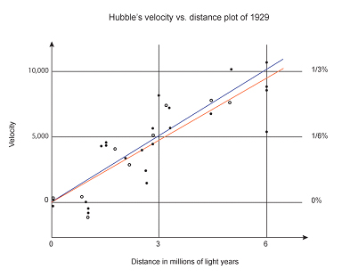
Edwin Hubble’s early published data are shown in Figure B.13.1. The first data (top), from 1929, were the basis for the initial announcement of the Hubble law, and correspondingly, the expansion of the Universe. In the figure, the solid circles and the blue line are for the galaxies treated individually, while the open circles and the red line combine the galaxies into groups. There were few galaxies in the sample and a wide scatter in the data, due largely to measurement errors. Hubble also mislabeled the y-axis ‘km’ rather than ‘km/s’. The 1931 data (bottom), collected with his assistant Milton Humason, demonstrate the Hubble Law far more convincingly, mainly by extending measurements to much more distant galaxies; most of the 1929 data are contained within the small box at the extreme lower left of the 1931 plot.

The values for the Hubble constant derived from the slopes of the lines in these plots were wrong by a large factor (about 10) due to several unrecognized systematic errors. Unknown at the time, there are different classes of Cepheid variables, and Hubble applied the period-luminosity law of one class to objects of the other. Hubble did not know about the cosmic distance ladder, so he had to improvise. For instance, in distant galaxies Cepheids were too faint for him to detect, forcing him to find (or invent) alternative ways of measuring the distances to those galaxies. Even now, when we look at the most distant galaxies visible in our most powerful telescopes, we cannot see the Cepheids in them because they are too faint. Hubble had no chance of seeing them in the 1920s.

This error was not corrected for many years and resulted in serious overestimates of the speed of expansion of the Universe—and correspondingly short age estimates for the Universe, as we will see.

Figure B.13.1: Hubble’s original data from 1929 (top) and Hubble and Humason’s data from 1931 (bottom). Solid circles and blue lines are data and fits for the galaxies treated individually, while the open circles and the red line in the top figure aggregate the data. Credit: NASA/SSU/Aurore Simonnet based on Hubble and Humason’s data.

One possible interpretation of a relation like Hubble’s, and the most obvious, is that it is due to the motions of galaxies through space. If we interpret the redshifts of galaxies as Doppler shifts, then we can convert redshifts into velocities through space. While the Doppler interpretation is obvious and easy to understand, it turns out not to be the correct interpretation. It is not consistent with other observations, which we will come to in a moment.